9.7 ROUGH DIELECTRIC BSDF
9.7 粗糙介电BSDF
We will now extend the microfacet approach from Section 9.6 to the case of rough dielectrics. This involves two notable changes: since dielectrics are characterized by both reflection and transmission, the model must be aware of these two separate components. In the case of transmission, Snell’s law will furthermore replace the law of reflection in the computation that determines the incident direction.
我们现在将把 9.6 节中的微面方法扩展到粗糙电介质的情况。这涉及两个显着的变化:由于电介质具有反射和透射的特征,因此模型必须了解这两个独立的组件。在透射的情况下,斯涅尔定律将在确定入射方向的计算中进一步取代反射定律。
Figure 9.32 shows the dragon rendered with the Torrance–Sparrow model and both reflection and transmission.
图 9.32 显示了使用 Torrance-Sparrow 模型以及反射和透射渲染的龙。
As before, we will begin by characterizing the probability density of generated samples. The implied BSDF then directly follows from this density and the sequence of events encapsulated by a scattering interaction: visible normal sampling, reflection or refraction, and attenuation by the Fresnel and masking terms.
和以前一样,我们将从表征生成样本的概率密度开始。然后,隐含的 BSDF 直接从该密度和由散射相互作用封装的事件序列得出:可见法线采样、反射或折射,以及菲涅耳和掩蔽项的衰减。
Rough Dielectric PDF
粗糙电介质 PDF
The density evaluation occurs in the following fragment that we previously omitted during the discussion of the smooth dielectric case.
密度评估发生在我们之前在讨论光滑介电情况时省略的以下片段中。
〈Evaluate sampling PDF of rough dielectric BSDF〉 ≡ 〈Compute generalized half vector wm 588〉 〈Discard backfacing microfacets 588〉 〈Determine Fresnel reflectance of rough dielectric boundary 588〉 〈Compute probabilities pr and pt for sampling reflection and transmission 564〉 〈Return PDF for rough dielectric 589〉 |
566 |
We now turn to the generalized half-direction vector, whose discussion requires a closer look at Snell’s law (Equation (9.2)) relating the elevation and azimuth of the incident and outgoing directions at a refractive interface:
我们现在转向广义半方向矢量,其讨论需要仔细研究斯涅尔定律(方程(9.2)),该定律涉及折射界面处入射和出射方向的仰角和方位角:
ηo sin θo = ηi sin θi and ϕo = ϕi + π.
η o sin θ o = η sin θ 且 phi o = phi + π。
Since the refraction takes place at the level of the microgeometry, all of these angles are to be understood within a coordinate frame aligned with the microfacet normal ωm. Recall also that the sines in the first equation refer to the length of the tangential component of ωi and ωo perpendicular to ωm.
由于折射发生在微观几何水平上,因此所有这些角度都应在与微面法线 ω m 对齐的坐标系内理解。还记得第一个方程中的正弦是指 ω 和垂直于 ω m 的 ω o 的切向分量的长度。
A generalized half-direction vector builds on this observation by scaling and adding these directions to cancel out the tangential components, which yields the surface normal responsible for a particular refraction after normalization. It is defined as
广义半方向矢量建立在该观察的基础上,通过缩放和添加这些方向来抵消切向分量,从而在归一化后产生负责特定折射的表面法线。它被定义为

where η = ηi/ηo is the relative index of refraction toward the sampled direction ωi. The reflective case is trivially subsumed, since ηi = ηo when no refraction takes place. The next fragment implements this computation, including handling of invalid configurations (e.g., perfectly grazing incidence) where both the BSDF and its sampling density evaluate to zero.
其中 η = η/η o 是朝向采样方向 ω 的相对折射率。反射情况被简单地包含在内,因为当没有发生折射时 η = η o 。下一个片段实现此计算,包括处理无效配置(例如,完美的掠射发生率),其中 BSDF 及其采样密度评估为零。
〈Compute generalized half vector wm〉 ≡ Float cosTheta_o = CosTheta(wo), cosTheta_i = CosTheta(wi); bool reflect = cosTheta_i * cosTheta_o > 0; float etap = 1; if (!reflect) etap = cosTheta_o > 0 ? eta : (1 / eta); Vector3f wm = wi * etap + wo; if (cosTheta_i == 0 || cosTheta_o == 0 || LengthSquared(wm) == 0) return {}; wm = FaceForward(Normalize(wm), Normal3f(0, 0, 1)); |
587, 589 |
The last line reflects an important implementation detail: with the previous definition in Equation (9.34), ωm always points toward the denser medium, whereas pbrt uses the convention that micro- and macro-normal are consistently oriented (i.e., ωm · n > 0). In practice, we therefore compute the following modified half-direction vector, where n = (0, 0, 1) in local coordinates:
最后一行反映了一个重要的实现细节:根据方程(9.34)中的先前定义,ω m 始终指向较致密的介质,而 pbrt 使用微观法线和宏观法线一致定向的约定(即 ω m · n > 0)。因此,在实践中,我们计算以下修改后的半方向向量,其中局部坐标中的 n = (0, 0, 1):

Next, microfacets that are backfacing with respect to either the incident or outgoing direction do not contribute and must be discarded.
接下来,相对于入射或出射方向背面的微面没有贡献,必须被丢弃。
〈Discard backfacing microfacets〉 ≡ if (Dot(wm, wi) * cosTheta_i < 0 || Dot(wm, wo) * cosTheta_o < 0) return {}; |
587, 589 |
Given ωm, we can evaluate the Fresnel reflection and transmission terms using the specialized dielectric evaluation of the Fresnel equations.
给定 ω m ,我们可以使用菲涅尔方程的专门介电评估来评估菲涅尔反射和传输项。
〈Determine Fresnel reflectance of rough dielectric boundary〉 ≡ Float R = FrDielectric(Dot(wo, wm), eta); Float T = 1 - R; |
587 |
CosTheta() 107
第 107 章
DielectricBxDF::eta 563
电介质BxDF::eta 563
Dot() 89
点() 89
FaceForward() 94
第 94 章
Float 23
浮法23
FrDielectric() 557
LengthSquared() 87
长度平方() 87
Normal3f 94
普通3f 94
Normalize() 88
标准化() 88
Vector3f 86
矢量3f 86
We now have the values necessary to compute the PDF for ωi, which depends on whether it reflects or transmits at the surface.
现在我们有了计算 ω 的 PDF 所需的值,这取决于它是在表面反射还是透射。
〈Return PDF for rough dielectric〉 ≡ Float pdf; if (reflect) { 〈Compute PDF of rough dielectric reflection 589〉 } else { 〈Compute PDF of rough dielectric transmission 589〉 } return pdf; |
587 |
As before, the bijective mapping between ωm and ωi provides a change of variables whose Jacobian determinant is crucial so that we can correctly deduce the probability density of sampled directions ωi. The derivation is more involved in the refractive case; see the “Further Reading” section for pointers to its derivation. The final determinant is given by
和之前一样,ω m 和 ω 之间的双射映射提供了变量的变化,其雅可比行列式至关重要,以便我们可以正确推导采样方向 ω 的概率密度。推导更多地涉及屈光情况;请参阅“进一步阅读”部分以获取其推导的指针。最终的行列式由下式给出
Once more, this relationship makes it possible to evaluate the probability per unit solid angle of the sampled incident directions ωi obtained through the combination of visible normal sampling and scattering:
再次,这种关系使得可以评估通过可见法向采样和散射相结合获得的采样入射方向 ω 的每单位立体角的概率:

The following fragment implements this computation, while additionally accounting for the discrete probability pt / (pr + pt) of sampling the transmission component.
以下片段实现了此计算,同时另外考虑了对传输分量进行采样的离散概率 pt / (pr + pt)。
〈Compute PDF of rough dielectric transmission〉 ≡ Float denom = Sqr(Dot(wi, wm) + Dot(wo, wm) / etap); Float dwm_dwi = AbsDot(wi, wm) / denom; pdf = mfDistrib.PDF(wo, wm) * dwm_dwi * pt / (pr + pt); |
589, 591 |
Finally, the density of the reflection component agrees with the model used for conductors but for the additional discrete probability pr / (pr + pt) of choosing the reflection component.
最后,反射分量的密度与用于导体的模型一致,但选择反射分量的附加离散概率 pr / (pr + pt) 除外。
〈Compute PDF of rough dielectric reflection〉 ≡ pdf = mfDistrib.PDF(wo, wm) / (4 * AbsDot(wo, wm)) * pr / (pr + pt); |
589, 591 |
Rough Dielectric BSDF
粗糙电介质 BSDF
BSDF evaluation is similarly split into reflective and transmissive components.
BSDF 评估同样分为反射部分和透射部分。
〈Evaluate rough dielectric BSDF〉 ≡ 〈Compute generalized half vector wm 588〉 〈Discard backfacing microfacets 588〉 Float F = FrDielectric(Dot(wo, wm), eta); if (reflect) { 〈Compute reflection at rough dielectric interface 590〉 } else { 〈Compute transmission at rough dielectric interface 590〉 } |
566 |
AbsDot() 90
绝对点() 90
DielectricBxDF::eta 563
电介质BxDF::eta 563
DielectricBxDF::mfDistrib 563
电介质BxDF::mfDistrib 563
Dot() 89
点() 89
Float 23
浮法23
FrDielectric() 557
Sqr() 1034
平方() 1034
TrowbridgeReitzDistribution::PDF() 579
特罗布里奇ReitzDistribution::PDF() 579
The reflection component follows the approach used for conductors in the fragment 〈Evaluate rough conductor BRDF〉:
反射分量遵循片段<评估粗糙导体 BRDF> 中用于导体的方法:
〈Compute reflection at rough dielectric interface〉 ≡ return SampledSpectrum(mfDistrib.D(wm) * mfDistrib.G(wo, wi) * F / std::abs(4 * cosTheta_i * cosTheta_o)); |
589 |
For the transmission component, we can again derive the effective scattering distribution by equating a single-sample Monte Carlo estimate of the rendering equation with the product of Fresnel transmission, masking, and the incident radiance. This results in the equation
对于透射分量,我们可以通过将渲染方程的单样本蒙特卡罗估计与菲涅尔透射、掩蔽和入射辐射率的乘积等同起来,再次导出有效散射分布。这导致方程

Substituting the PDF from Equation (9.37) and solving for the BTDF ft(p, ωo, ωi) results in
将 PDF 代入方程 (9.37) 并求解 BTDF f t (p, ω o , ω) 结果为

Finally, inserting the definition of the visible normal distribution from Equation (9.23) and switching to the more accurate bidirectional masking-shadowing factor G yields
最后,插入方程(9.23)中可见正态分布的定义并切换到更准确的双向掩蔽-阴影因子 G,得出

The next fragment implements this expression. It also incorporates the earlier orientation test and handling of non-symmetric scattering that was previously encountered in the perfect specular case (Section 9.5.2).
下一个片段实现了这个表达式。它还结合了先前在完美镜面反射情况下遇到的非对称散射的定向测试和处理(第 9.5.2 节)。
〈Compute transmission at rough dielectric interface〉 ≡ Float denom = Sqr(Dot(wi, wm) + Dot(wo, wm)/etap) * cosTheta_i * cosTheta_o; Float ft = mfDistrib.D(wm) * (1 - F) * mfDistrib.G(wo, wi) * std::abs(Dot(wi, wm) * Dot(wo, wm) / denom); 〈Account for non-symmetry with transmission to different medium 571〉 return SampledSpectrum(ft); |
589 |
Rough Dielectric Sampling
粗介电采样
Sampling proceeds by drawing a microfacet normal from the visible normal distribution, computing the Fresnel term, and stochastically selecting between reflection and transmission.
通过从可见正态分布中绘制微面法线、计算菲涅耳项并在反射和透射之间随机选择来进行采样。
〈Sample rough dielectric BSDF〉 ≡ Vector3f wm = mfDistrib.Sample_wm(wo, u); Float R = FrDielectric(Dot(wo, wm), eta); Float T = 1 - R; 〈Compute probabilities pr and pt for sampling reflection and transmission 564〉 Float pdf; if (uc < pr / (pr + pt)) { 〈Sample reflection at rough dielectric interface 591〉 } else { 〈Sample transmission at rough dielectric interface 591〉 } |
564 |
Once again, handling of the reflection component is straightforward and mostly matches the case for conductors except for extra factors that arise due to the discrete choice between reflection and transmission components.
再次强调,反射分量的处理非常简单,并且除了由于反射和传输分量之间的离散选择而产生的额外因素之外,大部分与导体的情况匹配。
DielectricBxDF::mfDistrib 563
电介质BxDF::mfDistrib 563
Dot() 89
点() 89
Float 23
浮法23
FrDielectric() 557
SampledSpectrum 171
采样频谱 171
Sqr() 1034
平方() 1034
TrowbridgeReitzDistribution::D() 575
第 575 章
TrowbridgeReitzDistribution::G() 578
第 578 章
TrowbridgeReitzDistribution::Sample_wm() 580
第580章
Vector3f 86
矢量3f 86
〈Sample reflection at rough dielectric interface〉 ≡ Vector3f wi = Reflect(wo, wm); if (!SameHemisphere(wo, wi)) return {}; 〈Compute PDF of rough dielectric reflection 589〉 SampledSpectrum f(mfDistrib.D(wm) * mfDistrib.G(wo, wi) * R / (4 * CosTheta(wi) * CosTheta(wo))); return BSDFSample(f, wi, pdf, BxDFFlags::GlossyReflection); |
590 |
The transmission case invokes Refract() to determine wi. A subsequent test excludes inconsistencies that can rarely arise due to the approximate nature of floating-point arithmetic. For example, Refract() may sometimes indicate a total internal reflection configuration, which is inconsistent as the transmission component should not have been sampled in this case.
传输案例调用 Refract() 来确定 wi。随后的测试排除了由于浮点运算的近似性质而很少出现的不一致情况。例如,Refract() 有时可能指示全内反射配置,这是不一致的,因为在这种情况下不应对传输分量进行采样。
〈Sample transmission at rough dielectric interface〉 ≡ Float etap; Vector3f wi; bool tir = !Refract(wo, (Normal3f)wm, eta, &etap, &wi); if (SameHemisphere(wo, wi) || wi.z == 0 || tir) return {}; 〈Compute PDF of rough dielectric transmission 589〉 〈Evaluate BRDF and return BSDFSample for rough transmission 591〉 |
590 |
The last step evaluates the BTDF from Equation (9.40) and packs the sample information into a BSDFSample.
最后一步根据方程 (9.40) 评估 BTDF,并将样本信息打包到 BSDFSample 中。
〈Evaluate BRDF and return BSDFSample for rough transmission〉 ≡ SampledSpectrum ft(T * mfDistrib.D(wm) * mfDistrib.G(wo, wi) * std::abs(Dot(wi, wm) * Dot(wo, wm) / (CosTheta(wi) * CosTheta(wo) * denom))); 〈Account for non-symmetry with transmission to different medium 571〉 return BSDFSample(ft, wi, pdf, BxDFFlags::GlossyTransmission, etap); |
591 |
9.8 MEASURED BSDFs
9.8 测量的 BSDF
The reflection models introduced up to this point represent index of refraction changes at smooth and rough boundaries, which constitute the basic building blocks of surface appearance. More complex materials (e.g., paint on primer, metal under a layer of enamel) can sometimes be approximated using multiple interfaces with participating media between them; the layered material model presented in Section 14.3 is based on that approach.
到目前为止介绍的反射模型代表了光滑和粗糙边界处的折射率变化,它们构成了表面外观的基本构建块。更复杂的材料(例如,底漆上的油漆、搪瓷层下的金属)有时可以使用多个界面以及它们之间的参与介质来近似;第 14.3 节中介绍的分层材料模型基于该方法。
However, many real-world materials are beyond the scope of even such layered models. Examples include:
然而,许多现实世界的材料甚至超出了这种分层模型的范围。示例包括:
- Materials characterized by wave-optical phenomena that produce striking directionally varying coloration. Examples include iridescent paints, insect wings, and holographic paper.
以波光现象为特征的材料,可产生引人注目的方向变化的颜色。例如虹彩涂料、昆虫翅膀和全息纸。 - Materials with rough interfaces. In pbrt, we have chosen to model such surfaces using microfacet theory and the Trowbridge–Reitz distribution. However, it is important to remember that both of these are models that generally do not match real-world behavior perfectly.
界面粗糙的材料。在 pbrt 中,我们选择使用微面理论和 Trowbridge-Reitz 分布对此类表面进行建模。然而,重要的是要记住,这两种模型通常都无法完美匹配现实世界的行为。 - Surfaces with non-standard microstructure. For example, a woven fabric composed of two different yarns looks like a surface from a distance, but its directional intensity and color variation are not well-described by any standard BRDF model due to the distinct reflectance properties of fiber-based microgeometry.
具有非标准微观结构的表面。例如,由两种不同纱线组成的机织织物从远处看就像一个表面,但由于基于纤维的微观几何形状具有独特的反射特性,任何标准 BRDF 模型都无法很好地描述其方向强度和颜色变化。
BSDFSample 541
BSDF样本 541
BxDFFlags::GlossyReflection 539
BxDFFlags::光泽反射 539
BxDFFlags::GlossyTransmission 539
BxDFFlags::光泽传输 539
CosTheta() 107
第 107 章
DielectricBxDF::mfDistrib 563
电介质BxDF::mfDistrib 563
Dot() 89
点() 89
Float 23
浮法23
Normal3f 94
普通3f 94
Reflect() 552
反射()552
Refract() 554
折射() 554
SameHemisphere() 538
SampledSpectrum 171
采样频谱 171
TrowbridgeReitzDistribution::D() 575
第 575 章
TrowbridgeReitzDistribution::G() 578
第 578 章
Vector3f 86
矢量3f 86
Instead of developing numerous additional specialized BxDFs, we will now pursue another way of reproducing such challenging materials in a renderer: by interpolating measurements of real-world material samples to create a data-driven reflectance model. The resulting MeasuredBxDF only models surface reflection, though the approach can in principle generalize to transmission as well.
我们现在将不再开发大量额外的专用 BxDF,而是寻求另一种在渲染器中再现此类具有挑战性的材质的方法:通过对现实世界材质样本的测量进行插值来创建数据驱动的反射率模型。所得的 MeasuredBxDF 仅模拟表面反射,但该方法原则上也可以推广到传输。
〈MeasuredBxDF Definition〉 ≡
〈测量dBxDF定义〉 ≡
class MeasuredBxDF {
类MeasuredBxDF {
public:
民众:
〈MeasuredBxDF Public Methods〉
〈MeasuredBxDF 公共方法〉
private:
私人的:
〈MeasuredBxDF Private Methods 601〉
〈MeasuredBxDF 私有方法 601〉
〈MeasuredBxDF Private Members 600〉
〈实测dBxDF私人会员600〉
};
Measuring reflection in a way that is practical while producing information in a form that is convenient for rendering is a challenging problem. We begin by explaining these challenges for motivation.
以实用的方式测量反射,同时以方便渲染的形式生成信息是一个具有挑战性的问题。我们首先解释这些激励挑战。
Consider the task of measuring the BRDF of a sheet of brushed aluminum: we could illuminate a sample of the material from a set of n incident directions  with k = 1, … , n and use some kind of sensor (e.g., a photodiode) to record the reflected light scattered along a set of m outgoing directions
  with l = 1, … , m. These n × m measurements could be stored on disk and interpolated at runtime to approximate the BRDF at intermediate configurations (θi, ϕi, θo, ϕo). However, closer scrutiny of such an approach reveals several problems:
考虑测量拉丝铝板的 BRDF 的任务:我们可以从一组 n 个入射方向 照射材料样本,其中 k = 1, … , n 并使用某种传感器(例如,光电二极管)记录沿一组 m 个出射方向 散射的反射光,其中 l = 1, … , m。这些 n × m 测量值可以存储在磁盘上,并在运行时进行插值,以近似中间配置(θ、 Φ、 θ o 、 Φ o )下的 BRDF。然而,对这种方法的仔细审查揭示了几个问题:
- BSDFs of polished materials are highly directionally peaked. Perturbing the incident or outgoing direction by as little as 1 degree can change the measured reflectance by orders of magnitude. This implies that the set of incident and outgoing directions must be sampled fairly densely.
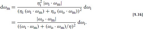
抛光材料的 BSDF 具有高度方向性的峰值。只要扰动入射或出射方向 1 度,就能将测量到的反射率改变几个数量级。这意味着必须对入射和出射方向集进行相当密集的采样。 - Accurate positioning in spherical coordinates is difficult to perform by hand and generally requires mechanical aids. For this reason, such measurements are normally performed using a motorized gantry known as a goniophotometer or gonioreflectometer. Figure 9.33 shows two examples of such machines. Light stages consisting of a rigid assembly of hundreds of LEDs around a sample are sometimes used to accelerate measurement, though at the cost of reduced directional resolution.
球面坐标中的精确定位很难用手执行,通常需要机械辅助。因此,此类测量通常使用称为测角光度计或测角反射计的电动龙门架进行。图 9.33 显示了此类机器的两个示例。有时使用由围绕样品的数百个 LED 刚性组件组成的光台来加速测量,但代价是方向分辨率降低。 - Sampling each direction using a 1 degree spacing in spherical coordinates requires roughly one billion sample points. Storing gigabytes of measurement data is possible but undesirable, yet the time that would be spent for a full measurement is even more problematic: assuming that the goniophotometer can reach a configuration (θi, ϕi, θo, ϕo) within 1 second (a reasonable estimate for the devices shown in Figure 9.33), over 34 years of sustained operation would be needed to measure a single material.
在球坐标中使用 1 度间距对每个方向进行采样大约需要 10 亿个采样点。存储千兆字节的测量数据是可能的,但并不可取,但完整测量所花费的时间甚至更成问题:假设测角光度计可以达到配置 (θ, Φ, θ o , Φ < b1>)在 1 秒内(对图 9.33 中所示设备的合理估计),需要持续运行超过 34 年才能测量单一材料。
In sum, the combination of high-frequency signals, the 4D domain of the BRDF, and the curse of dimensionality conspire to make standard measurement approaches all but impractical.
总之,高频信号、BRDF 的 4D 域和维数灾难的结合使标准测量方法几乎不切实际。
BxDF 538
B×DF 538
MeasuredBxDF 592
测量dBxDF 592
While there is no general antidote against the curse of dimensionality, the previous example involving a dense discretization of the 4D domain is clearly excessive. For example, peaked BSDFs that concentrate most of their energy into a small set of angles tend to be relatively smooth away from the peak. Figure 9.34 shows how a more specialized sample placement that is informed by the principles of specular reflection can drastically reduce the number of sample points that are needed to obtain a desired level of accuracy. Figure 9.35 shows how the roughness of the surface affects the desired distribution of samples—for example, smooth surfaces allow sparse sampling outside of the specular lobe.
虽然没有针对维数灾难的通用解药,但前面涉及 4D 域密集离散化的示例显然有些过分。例如,将大部分能量集中到一小部分角度的峰值 BSDF 往往会相对平滑地远离峰值。图 9.34 显示了根据镜面反射原理进行的更专业的样本放置如何能够大大减少获得所需精度水平所需的样本点数量。图 9.35 显示了表面的粗糙度如何影响所需的样本分布,例如,光滑的表面允许在镜面波瓣之外进行稀疏采样。
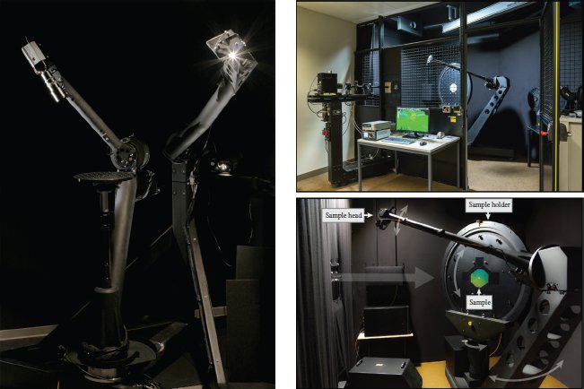
Figure 9.33: Specialized Hardware for BSDF Acquisition. The term goniophotometer (or gonioreflectometer) refers to a typically motorized platform that can simultaneously illuminate and observe a material sample from arbitrary pairs of directions. The device on the left (at Cornell University, built by Cyberware Inc., image courtesy of Steve Marschner) rotates camera (2 degrees of freedom) and light arms (1 degree of freedom) around a centered sample pedestal that can also rotate about its vertical axis. The device on the right (at EPFL, built by pab advanced technologies Ltd) instead uses a static light source and a rotating sensor arm (2 degrees of freedom). The vertical material sample holder then provides 2 rotational degrees of freedom to cover the full 4D domain of the BSDF.
图 9.33:用于 BSDF 采集的专用硬件。术语“测角光度计”(或“测角反射计”)是指一种典型的机动平台,可以从任意对方向同时照明和观察材料样本。左侧的设备(位于康奈尔大学,由 Cyberware Inc. 建造,图片由 Steve Marschner 提供)围绕中心样品基座旋转相机(2 个自由度)和光臂(1 个自由度),该样品基座也可以绕其自身旋转垂直轴。右侧的设备(位于 EPFL,由 PAB Advanced Technologies Ltd 制造)改为使用静态光源和旋转传感器臂(2 个自由度)。然后,垂直材料样品支架提供 2 个旋转自由度,以覆盖 BSDF 的完整 4D 域。
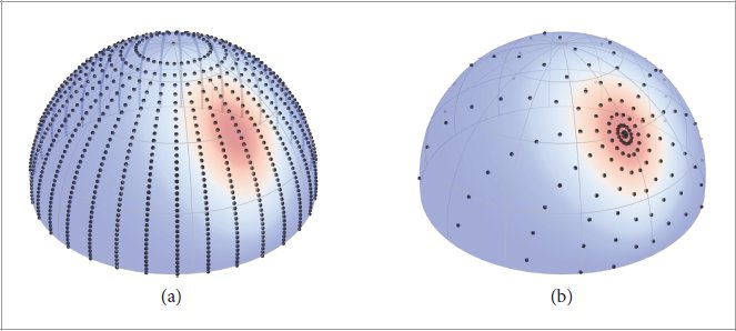
Figure 9.34: Adaptive BRDF Sample Placement. (a) Regular sampling of the incident and outgoing directions is a prohibitively expensive way of measuring and storing BRDFs due to the curse of dimensionality (here, only 2 of the 4 dimensions are shown). (b) A smaller number of samples can yield a more accurate interpolant if their placement is informed by the material’s reflectance behavior.
图 9.34:自适应 BRDF 样本放置。 (a) 由于维度灾难(此处仅显示 4 个维度中的 2 个),定期对入射和出射方向进行采样是一种极其昂贵的测量和存储 BRDF 的方法。 (b) 如果样本的位置由材料的反射率行为决定,则较少数量的样本可以产生更准确的插值。
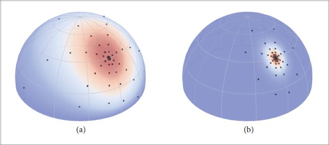
Figure 9.35: The Effect of Surface Roughness on Adaptive BRDF Sample Placement. The two plots visualize BRDF values of two materials with different roughnesses for varying directions ωi and fixed ωo. Circles indicate adaptively chosen measurement locations, which are used to create the interpolant implemented in the MeasuredBxDF class. (a) The measurement locations broadly cover the hemisphere given a relatively rough material. (b) For a more specular material the samples are concentrated in the region around the specular peak. Changing the outgoing direction moves the specular peak; hence the sample locations must depend on ωo.
图 9.35:表面粗糙度对自适应 BRDF 样本放置的影响。这两个图可视化了两种具有不同粗糙度的材料对于不同方向 ω 和固定 ω o 的 BRDF 值。圆圈表示自适应选择的测量位置,用于创建在 MeasuredBxDF 类中实现的插值。 (a) 考虑到材料相对粗糙,测量位置广泛覆盖半球。 (b) 对于更镜面反射的材料,样本集中在镜面反射峰周围的区域。改变出射方向会移动镜面反射峰值;因此样本位置必须取决于 ω o 。
The MeasuredBxDF therefore builds on microfacet theory and the distribution of visible normals to create a more efficient physically informed sampling pattern. The rationale underlying this choice is that while microfacet theory may not perfectly predict the reflectance of a specific material, it can at least approximately represent how energy is (re-)distributed throughout the 4D domain. Applying it enables the use of a relatively coarse set of measurement locations that suffice to capture the function’s behavior.
因此,MeasuredBxDF 基于微面理论和可见法线的分布,以创建更有效的物理信息采样模式。这一选择的基本原理是,虽然微面理论可能无法完美预测特定材料的反射率,但它至少可以近似地表示能量在整个 4D 域中(重新)分布的方式。应用它可以使用一组相对粗糙的测量位置,足以捕获函数的行为。
Concretely, the method works by transforming regular grid points using visible normal sampling (Section 9.6.4) and performing a measurement at each sampled position. If the microfacet sampling routine is given by a function R : S2 × [0, 1]2 → S2 and u(k) with k = 1, … , n denotes input samples arranged on a grid covering the 2D unit square, then we have a sequence of measurements M(k):
具体来说,该方法的工作原理是使用可见法线采样(第 9.6.4 节)转换规则网格点,并在每个采样位置执行测量。如果微面采样例程由函数 R 给出: S 2 × [0, 1] 2 → S 2 和 u (k) 其中 k = 1, … , n 表示排列在覆盖 2D 单位正方形的网格上的输入样本,那么我们有一个测量序列 M (k) :

where fr(ωo, ωi) refers to the real-world BRDF of a material sample, as measured by a goniophotometer (or similar device) in directions ωo and ωi = R(ωo, u(k)). This process must be repeated for different values of ωo to also capture variation in the other direction argument. Evaluating the BRDF requires the inverse R−1 of the transformation, which yields a position on [0, 1]2 that can be used to interpolate the measurements M(k). Figure 9.36 illustrates both directions of this mapping.
其中 f r (ω o , ω) 是指材料样本的现实世界 BRDF,由测角光度计(或类似设备)沿 ω o , u (k) )。必须针对不同的 ω o 值重复此过程,以捕获另一个方向参数的变化。评估 BRDF 需要变换的逆 R −1 ,这会产生 [0, 1] 2 上的位置,可用于插值测量值 M (k) .图 9.36 说明了该映射的两个方向。
This procedure raises several questions: first, the non-random use of a method designed for Monte Carlo sampling may be unexpected. To see why this works, remember that the inversion method (Section 2.3) evaluates the inverse of a distribution’s cumulative distribution function (CDF). Besides being convenient for sampling, this inverse CDF can also be interpreted as a parameterization of the target domain from the unit square. This parameterization smoothly warps the domain so that regions with a high contribution occupy a correspondingly large amount of the unit square. The MeasuredBxDF then simply measures and stores BRDF values in these “improved” coordinates. Note that the material does not have to agree with microfacet theory for this warping to be valid, though the sampling pattern is much less efficient and requires a denser discretization when the material’s behavior deviates significantly.
这个过程提出了几个问题:首先,非随机使用为蒙特卡洛抽样设计的方法可能会出乎意料。要了解其原理,请记住反演方法(第 2.3 节)计算分布累积分布函数 (CDF) 的逆函数。除了方便采样之外,这种逆 CDF 还可以解释为单位平方对目标域的参数化。这种参数化平滑地扭曲域,使得具有高贡献的区域占据相应大量的单位正方形。然后,MeasuredBxDF 会简单地测量 BRDF 值并将其存储在这些“改进的”坐标中。请注意,材料不必符合微面理论才能使这种扭曲有效,尽管采样模式的效率要低得多,并且当材料的行为显着偏离时需要更密集的离散化。
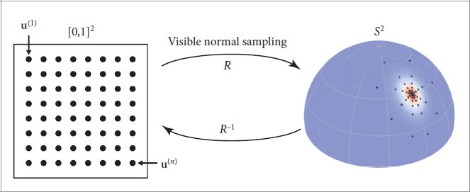
Figure 9.36: Visible Normal Sampling as a Parameterization. The MeasuredBxDF leverages visible normal sampling as a parameterization R of the unit sphere. Here, it is used in a deterministic fashion to transform a set of grid points u(k) with k = 1, … , n into spherical directions to be measured. Evaluating the resulting BRDF representation requires the inverse R−1 followed by linear interpolation within the regular grid of measurements.
图 9.36:作为参数化的可见正态采样。 MeasuredBxDF 利用可见法线采样作为单位球体的参数化 R。这里,它以确定性的方式将一组 k = 1, … , n 的网格点 u (k) 转换为要测量的球面方向。评估生成的 BRDF 表示需要逆 R −1 ,然后在规则测量网格内进行线性插值。
Another challenge is that parameterization guiding the measurement requires a microfacet approximation of the material, but such an approximation would normally be derived from an existing measurement. We will shortly show how to resolve this chicken-and-egg problem and assume for now that a suitable model is available.
另一个挑战是指导测量的参数化需要材料的微面近似,但这种近似通常是从现有的测量中得出的。我们很快就会展示如何解决这个先有鸡还是先有蛋的问题,并假设现在有一个合适的模型可用。
Measurement Through a Parameterization
通过参数化进行测量
A flaw of the reparameterized measurement sequence in Equation (9.41) is that the values M(k) may differ by many orders of magnitude, which means that simple linear interpolation between neighboring data points is unlikely to give satisfactory results. We instead use the following representation that transforms measurements prior to storage in an effort to reduce this variation:
等式(9.41)中重新参数化的测量序列的缺陷是值M (k) 可能相差多个数量级,这意味着相邻数据点之间的简单线性插值不太可能给出令人满意的结果。相反,我们使用以下表示在存储之前转换测量值,以减少这种变化:
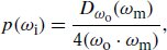
where ωi(k) = R(ωo, u(k)), and p(ωi(k)) denotes the density of direction ωi(k) according to visible normal sampling.
其中 ω (k) = R(ω o , u (k) ),p(ω (k) ) 表示方向 ω < 的密度b4>按照可见正常采样。
If fr was an analytic BRDF (e.g., a microfacet model) and u(k) a 2D uniform variate, then Equation (9.42) would simply be the weight of a Monte Carlo importance sampling strategy, typically with a carefully designed mapping R and density p that make this weight near-constant to reduce variance.
如果 f r 是解析 BRDF(例如微面模型),u (k) 是 2D 均匀变量,则方程 (9.42) 只是蒙特卡罗重要性采样的权重策略,通常采用精心设计的映射 R 和密度 p,使权重接近恒定以减少方差。
In the present context, fr represents real-world data, while p and R encapsulate a microfacet approximation of the material under consideration. We therefore expect M(k) to take on near-constant values when the material is well-described by a microfacet model, and more marked deviations otherwise. This can roughly be interpreted as measuring the difference (in a multiplicative sense) between the real world and the microfacet simplification. Figure 9.37 visualizes the effect of the transformation in Equation (9.42).
在当前上下文中,f r 表示真实世界的数据,而 p 和 R 封装了所考虑材料的微面近似值。因此,当材料被微面模型很好地描述时,我们期望 M (k) 呈现接近恒定的值,否则会有更明显的偏差。这可以粗略地解释为测量现实世界和微面简化之间的差异(在乘法意义上)。图 9.37 可视化了方程 (9.42) 中变换的效果。
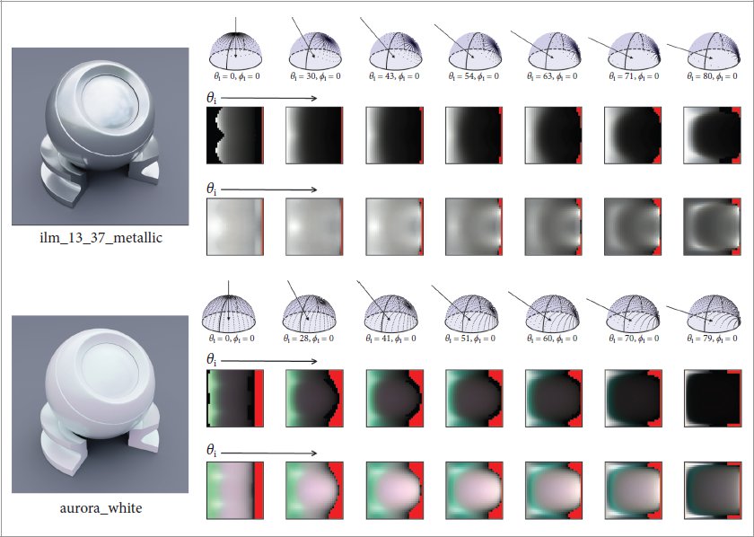
Figure 9.37: Reparameterized BRDF Visualization. This figure illustrates the representation of two material samples: a metallic sample swatch from the L3-37 robot in the film Solo: A Star Wars Story (Walt Disney Studios Motion Pictures) and a pearlescent vehicle vinyl wrap (TeckWrap International Inc.). Each column represents a measurement of a separate outgoing direction ωo. For both materials, the first row visualizes the measured directions ωi(k). The subsequent row plots the “raw” reparameterized BRDF of Equation (9.41), where each pixel represents one of the grid points u(k) ∈ [0, 1]2 identified with ωi(k). The final row shows transformed measurements corresponding to Equation (9.42) that are more uniform and easier to interpolate. Note that these samples are both isotropic, which is why a few measurements for different elevation angles suffice. In the anisotropic case, the (θo, ϕo) domain must be covered more densely.
图 9.37:重新参数化的 BRDF 可视化。该图展示了两种材料样本的表示:电影《游侠索罗:星球大战外传》(华特迪士尼影业电影公司)中 L3-37 机器人的金属样本样本和珠光车辆乙烯基包装(TeckWrap International Inc.)。每列表示单独的出射方向 ω o 的测量。对于这两种材料,第一行可视化测量的方向 ω (k) 。后续行绘制了方程 (9.41) 的“原始”重新参数化 BRDF,其中每个像素代表用 ω < 标识的网格点 u (k) ∈ [0, 1] 2 之一b4> 。最后一行显示了与方程 (9.42) 相对应的转换后的测量值,这些测量值更加均匀且更易于插值。请注意,这些样本都是各向同性的,这就是为什么对不同仰角进行一些测量就足够了。在各向异性情况下,(θ o , phi o ) 域必须被更密集地覆盖。
BRDF Evaluation
BRDF评估
Evaluating the data-driven BRDF requires the inverse of these steps. Suppose that M(·) implements an interpolation based on the grid of measurement points M(k). Furthermore, suppose that we have access to the inverse R−1(ωo, ωi) that returns the “random numbers” u that would cause visible normal sampling to generate a particular incident direction (i.e., R(ωo, u) = ωi). Accessing M(·) through R−1 then provides a spherical interpolation of the measurement data.
评估数据驱动的 BRDF 需要与这些步骤相反。假设 M(·) 基于测量点网格 M (k) 实现插值。此外,假设我们可以访问逆 R −1 (ω o , ω),它返回“随机数”u,这将导致可见法线采样生成特定的入射方向(即,R(ω o , u) = ω)。然后通过 R −1 访问 M(·) 提供测量数据的球形插值。
We must additionally multiply by the density p(ωi), and divide by the cosine factor5 to undo corresponding transformations introduced in Equation (9.42), which yields the final form of the data-driven BRDF:
我们还必须乘以密度 p(ω),并除以余弦因子 5 ,以撤消方程 (9.42) 中引入的相应变换,从而产生数据驱动的 BRDF 的最终形式:

Generalized Microfacet Model
广义微面模型
A major difference between the microfacet model underlying the ConductorBxDF and the approximation used here is that we replace the Trowbridge–Reitz model with an arbitrary data-driven microfacet distribution. This improves the model’s ability to approximate the material being measured. At the same time, it implies that previously used simplifications and analytic solutions are no longer available and must be revisited.
ConductorBxDF 底层的微面模型与此处使用的近似值之间的主要区别在于,我们用任意数据驱动的微面分布替换了 Trowbridge-Reitz 模型。这提高了模型近似被测量材料的能力。同时,这意味着以前使用的简化和解析解不再可用,必须重新审视。
We begin with the Torrance–Sparrow sampling density from Equation (9.28),
我们从方程 (9.28) 中的 Torrance-Sparrow 采样密度开始,
which references the visible normal sampling density Dω(ωm) from Equation (9.23). Substituting the definition of the masking function from Equation (9.18) into  and rearranging terms yields
它引用了方程(9.23)中的可见正常采样密度 D ω (ω m )。将等式 (9.18) 中掩蔽函数的定义代入 并重新排列项,得到
where
在哪里
provides a direction-dependent normalization of the visible normal distribution. For valid reflection directions (ωo · ωm > 0), the PDF of generated samples then simplifies to
提供可见正态分布的方向相关标准化。对于有效的反射方向 (ω o · ω m > 0),生成样本的 PDF 会简化为
Substituting this density into the BRDF from Equation (9.43) produces
将此密度代入方程 (9.43) 中的 BRDF 产生

The MeasuredBxDF implements this expression using data-driven representations of D(·) and σ(·).
MeasuredBxDF 使用 D(·) 和 σ(·) 的数据驱动表示来实现此表达式。
Finding the Initial Microfacet Model
寻找初始微面模型
We finally revisit the chicken-and-egg problem from before: practical measurement using the presented approach requires a suitable microfacet model—specifically, a microfacet distribution D(ωm). Yet it remains unclear how this distribution could be obtained without access to an already existing BRDF measurement.
我们最后重新审视之前的先有鸡还是先有蛋的问题:使用所提出的方法进行实际测量需要一个合适的微面模型,具体来说,一个微面分布 D(ω m )。然而,目前尚不清楚如何在不使用现有 BRDF 测量的情况下获得这种分布。
The key idea to resolve this conundrum is that the microfacet distribution D(ωm) is a 2D quantity, which means that it remains mostly unaffected by the curse of dimensionality. Acquiring this function is therefore substantially cheaper than a measurement of the full 4D BRDF.
解决这个难题的关键思想是微面分布 D(ω m ) 是一个二维量,这意味着它基本上不受维数灾难的影响。因此,获取此函数比完整 4D BRDF 的测量便宜得多。
Suppose that the material being measured perfectly matches microfacet theory in the sense that it is described by the Torrance–Sparrow BRDF from Equation (9.33). Then we can measure the material’s retroreflection (i.e., ωi = ωo = ω), which is given by
假设被测量的材料与微面理论完全匹配,因为它是由方程 (9.33) 中的 Torrance-Sparrow BRDF 描述的。然后我们可以测量材料的逆反射(即 ω = ω o = ω),其计算公式为

ConductorBxDF 560
导体BxDF 560
The last step of the above equation removes constant terms including the Fresnel reflectance and introduces the reasonable assumption that shadowing/masking is perfectly correlated given ωi = ωo and thus occurs only once. Substituting the definition of G1 from Equation (9.18) and rearranging yields the following relationship of proportionality:
上述方程的最后一步删除了包括菲涅尔反射率在内的常数项,并引入了合理的假设,即在给定 ω = ω o 的情况下,阴影/掩蔽完全相关,因此仅发生一次。将 G 1 的定义代入方程(9.18)并重新排列,得到以下比例关系:

This integral equation can be solved by measuring fr(p, ωj, ωj) for n directions ωj and using those measurements for initial guesses of D(ωj). A more accurate estimate of D can then be found using an iterative solution procedure where the estimated values of D are used to estimate the integrals on the right hand side of Equation (9.46) for all of the ωjs. This process quickly converges within a few iterations.
该积分方程可以通过测量 n 个方向 ω 的 f r (p, ω, ω) 并使用这些测量值作为 D(ω) 的初始猜测来求解。然后可以使用迭代求解过程找到 D 的更准确估计,其中 D 的估计值用于估计方程(9.46)右侧所有 ω 的积分。这个过程在几次迭代内很快收敛。
9.8.1 BASIC DATA STRUCTURES
9.8.1 基本数据结构
MeasuredBxDFData holds data pertaining to reflectance measurements and the underlying parameterization. Because the data for an isotropic BRDF is typically a few megabytes and the data for an anisotropic BRDF may be over 100, each measured BRDF that is used in the scene is stored in memory only once. As instances of MeasuredBxDF are created at surface intersections during rendering, they can then store just a pointer to the appropriate MeasuredBxDFData. Code not included here adds the ability to initialize instances of this type from binary .bsdf files containing existing measurements.6
MeasuredBxDFData 保存与反射率测量和底层参数化相关的数据。由于各向同性 BRDF 的数据通常为几兆字节,而各向异性 BRDF 的数据可能超过 100,因此场景中使用的每个测量的 BRDF 仅在内存中存储一次。由于 MeasuredBxDF 的实例是在渲染期间在表面相交处创建的,因此它们可以仅存储指向相应 MeasuredBxDFData 的指针。此处未包含的代码增加了从包含现有测量的二进制 .bsdf 文件初始化此类实例的能力。 6
〈MeasuredBxDFData Definition〉 ≡
〈测量dBxDF数据定义〉 ≡
struct MeasuredBxDFData {
结构体MeasuredBxDFData {
〈MeasuredBxDFData Public Members 598〉
〈MeasuredBxDFData 公共会员 598〉
};
Measured BRDFs are represented by spectral measurements at a set of discrete wavelengths that are stored in wavelengths. The actual measurements are stored in spectra.
测量的 BRDF 由存储在波长中的一组离散波长处的光谱测量值表示。实际测量结果存储在光谱中。
〈MeasuredBxDFData Public Members〉 ≡ pstd::vector<float> wavelengths; PiecewiseLinear2D<3> spectra; |
598 |
The template class PiecewiseLinear2D represents a piecewise-linear interpolant on the 2D unit square with samples arranged on a regular grid. The details of its implementation are relatively technical and reminiscent of other interpolants in this book; hence we only provide an overview of its capabilities and do not include its full implementation here.
模板类 PiecewiseLinear2D 表示 2D 单位正方形上的分段线性插值,样本排列在规则网格上。其实现的细节相对技术性强,让人想起本书中的其他插值器;因此,我们仅提供其功能的概述,并不包括其完整的实现。
The class is parameterized by a Dimension template parameter that extends the 2D interpolant to higher dimensions—for example, PiecewiseLinear2D<1> stores a 3D grid of values, and PiecewiseLinear2D<3> used above for spectra is a 5D quantity. The class provides three key methods:
该类通过 Dimension 模板参数进行参数化,该参数将 2D 插值扩展到更高维度 - 例如,PiecewiseLinear2D<1> 存储 3D 值网格,上面用于光谱的 PiecewiseLinear2D<3> 是 5D 量。该类提供了三个关键方法:
template <size_t Dimension> class PiecewiseLinear2D {
模板 类 PiecewiseLinear2D {
public:
民众:
Float Evaluate(Point2f pos, Float… params);
Float Evaluate(Point2f pos, Float…params);
PLSample Sample(Point2f u, Float… params);
PLSample 样本(Point2f u, Float... params);
PLSample Invert(Point2f p, Float… params);
PLSample Invert(Point2f p, Float... params);
};
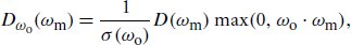
Figure 9.38: Three Measured BRDFs. (a) TeckWrap Amber Citrine vinyl wrapping film. (b) Purple acrylic felt. (c) Silk from an Indian sari with two colors of yarn.
图 9.38:三个测量的 BRDF。 (a) TeckWrap 琥珀黄水晶乙烯基包装膜。 (b) 紫色丙烯酸毡。 (c) 来自印度纱丽的丝绸,有两种颜色的纱线。
where PLSample is defined as
其中 PLSample 定义为
struct PLSample { Point2f p; Float pdf; };
struct PLSample { Point2f p;浮动pdf; };
Evaluate() takes a position pos ∈ [0, 1]2 and then additional Float parameters to perform a lookup using multidimensional linear interpolation according to the value of Dimension.
Evaluate() 采用位置 pos ∈ [0, 1] 2 ,然后附加 Float 参数,根据 Dimension 的值使用多维线性插值执行查找。
Sample() warps u ∈ [0, 1]2 via inverse transform sampling (i.e., proportional to the stored linear interpolant), returning both the sampled position on [0, 1]2 and the associated density as a PLSample. The additional parameters passed via params are used as conditional variables that restrict sampling to a 2D slice of a higher-dimensional function. For example, invoking the method PiecewiseLinear2D<3>::Sample() with a uniform 2D variate and parameters 0.1, 0.2, and 0.3 would importance sample the 2D slice I(0.1, 0.2, 0.3, ., .) of a pentalinear interpolant I.
Sample() 通过逆变换采样(即与存储的线性插值成比例)扭曲 u ∈ [0, 1] 2 ,返回 [0, 1] 2 以及作为 PLSample 的相关密度。通过 params 传递的附加参数用作条件变量,将采样限制为高维函数的 2D 切片。例如,使用统一 2D 变量和参数 0.1、0.2 和 0.3 调用方法 PiecewiseLinear2D<3>::Sample() 将对五线性插值的 2D 切片 I(0.1, 0.2, 0.3, ., .) 进行重要采样我。
Finally, Invert() implements the exact inverse of Sample(). Invoking it with the position computed by Sample() will recover the input u value up to rounding error.
最后,Invert() 实现了 Sample() 的精确逆操作。使用 Sample() 计算的位置调用它会将输入 u 值恢复到舍入误差。
Additional PiecewiseLinear1D instances are used to (redundantly) store the normal distribution D(ωm) in ndf, the visible normal distribution  parameterized by ωo = (θo, ϕo) in vndf, and the normalization constant σ(ωo) in sigma. The data structure also records whether the material is isotropic, in which case the dimensionality of some of the piecewise-linear interpolants can be reduced.
额外的 PiecewiseLinear1D 实例用于(冗余)存储 ndf 中的正态分布 D(ω m ),可见正态分布 参数化为 ω o = ( θ o 、 phi o )(以 vndf 表示)和归一化常数 σ(ω o ) (以 sigma 表示)。数据结构还记录材料是否是各向同性的,在这种情况下,可以降低一些分段线性插值的维数。
〈MeasuredBxDFData Public Members〉 +≡ PiecewiseLinear2D<0> ndf; PiecewiseLinear2D<2> vndf; PiecewiseLinear2D<0> sigma; bool isotropic; |
598 |
Following these preliminaries, we can now turn to evaluating the measured BRDF for a pair of directions. See Figure 9.38 for examples of the variety of types of reflection that the measured representation can reproduce.
完成这些准备工作后,我们现在可以转向评估两个方向的测量 BRDF。有关测量表示可以再现的各种反射类型的示例,请参见图 9.38。
PiecewiseLinear2D 598
分段线性二维 598
The only information that must be stored as MeasuredBxDF member variables in order to implement the BxDF interface methods is a pointer to the BRDF measurement data and the set of wavelengths at which the BRDF is to be evaluated.
为了实现 BxDF 接口方法,必须存储为 MeasuredBxDF 成员变量的唯一信息是指向 BRDF 测量数据和要评估 BRDF 的波长集的指针。
〈MeasuredBxDF Private Members〉 ≡ const MeasuredBxDFData *brdf; SampledWavelengths lambda; |
592 |
BRDF evaluation then follows the approach described in Equation (9.45).
然后,BRDF 评估遵循公式 (9.45) 中描述的方法。
〈MeasuredBxDF Method Definitions〉 ≡
〈MeasuredBxDF 方法定义〉 ≡
SampledSpectrum MeasuredBxDF::f(Vector3f wo, Vector3f wi,
采样频谱测量dBxDF::f(Vector3f wo, Vector3f wi,
TransportMode mode) const {
TransportMode 模式) const {
〈Check for valid reflection configurations 600〉
〈检查有效的反射配置600〉
〈Determine half-direction vector ωm 600〉
〈确定半方向向量 ω m 600〉
〈Map ωo and ωm to the unit square [0, 1]2〉
〈将 ω o 和 ω m 映射到单位正方形 [0, 1] 2 〉
〈Evaluate inverse parameterization R−1 601〉
〈求逆参数化 R −1 601〉
〈Evaluate spectral 5D interpolant 601〉
〈评估光谱5D插值601〉
〈Return measured BRDF value 601〉
〈返回测量的BRDF值601〉
}
Zero reflection is returned if the specified directions correspond to transmission through the surface. Otherwise, the directions ωi and ωo are mirrored onto the positive hemisphere if necessary.
如果指定方向对应于通过表面的透射,则返回零反射。否则,如有必要,方向 ω 和 ω o 将镜像到正半球上。
〈Check for valid reflection configurations〉 ≡ if (!SameHemisphere(wo, wi)) return SampledSpectrum(0); if (wo.z < 0) { wo = -wo; wi = -wi; } |
600 |
The next code fragment determines the associated microfacet normal and handles an edge case that occurs in near-grazing configurations.
下一个代码片段确定关联的微面法线并处理近掠配置中发生的边缘情况。
〈Determine half-direction vector ωm〉 ≡ Vector3f wm = wi + wo; if (LengthSquared(wm) == 0) return SampledSpectrum(0); wm = Normalize(wm); |
600 |
A later step requires that ωo and ωm are mapped onto the unit square [0, 1]2, which we do in two steps: first, by converting the directions to spherical coordinates, which are then further transformed by helper methods theta2u() and phi2u().
后面的步骤要求将 ω o 和 ω m 映射到单位正方形 [0, 1] 2 上,我们分两步进行:首先,通过将方向转换为球面坐标,然后通过辅助方法 theta2u() 和 phi2u() 进一步转换。
In the isotropic case, the mapping used for ωm subtracts ϕo from ϕm, which allows the stored tables to be invariant to rotation about the surface normal. This may cause the second dimension of u_wm to fall out of the [0, 1] interval; a subsequent correction fixes this using the periodicity of the azimuth parameter.
在各向同性情况下,用于 ω m 的映射从 phi m 中减去 phi o ,这使得存储的表格对于围绕表面法线的旋转保持不变。这可能会导致u_wm的第二维落在[0, 1]区间之外;随后的修正使用方位角参数的周期性来修复这个问题。
LengthSquared() 87
长度平方() 87
MeasuredBxDFData 598
测量的 dBxDF 数据 598
Normalize() 88
标准化() 88
SameHemisphere() 538
SampledSpectrum 171
采样频谱 171
SampledWavelengths 173
采样波长 173
TransportMode 571
运输方式 571
Vector3f 86
矢量3f 86
〈Map ωo and ωm to the unit square [0, 1]2〉 ≡
〈将 ω o 和 ω m 映射到单位正方形 [0, 1] 2 〉 ≡
Float theta_o = SphericalTheta(wo), phi_o = std::atan2(wo.y, wo.x);
浮点 theta_o = SphericalTheta(wo), phi_o = std::atan2(wo.y, wo.x);
Float theta_m = SphericalTheta(wm), phi_m = std::atan2(wm.y, wm.x);
浮点 theta_m = SphericalTheta(wm), phi_m = std::atan2(wm.y, wm.x);
Point2f u_wo(theta2u(theta_o), phi2u(phi_o));
Point2f u_wm(theta2u(theta_m), phi2u(brdf->isotropic ? (phi_m - phi_o) :
Point2f u_wm(theta2u(theta_m), phi2u(brdf->各向同性?(phi_m - phi_o) :
phi_m));
u_wm[1] = u_wm[1] - pstd::floor(u_wm[1]);
The two helper functions encapsulate an implementation detail of the storage representation. The function phi2u() uniformly maps [−π, π] onto [0, 1], while theta2u() uses a nonlinear transformation that places more resolution near θ ≈ 0 to facilitate storing the microfacet distribution of highly specular materials.
这两个辅助函数封装了存储表示的实现细节。函数 phi2u() 将 [−π, π] 均匀映射到 [0, 1],而 theta2u() 使用非线性变换,将更高的分辨率置于 θ ≈ 0 附近,以便于存储高镜面材料的微面分布。
〈MeasuredBxDF Private Methods〉 ≡ static Float theta2u(Float theta) { return std::sqrt(theta * (2 / Pi)); } static Float phi2u(Float phi) { return phi * (1 / (2 * Pi)) + .5f; } |
592 |
With this information at hand, we can now evaluate the inverse parameterization to determine the sample values ui.p that would cause visible normal sampling to generate the current incident direction (i.e., R(ωo, u) = ωi).
有了这些信息,我们现在可以评估逆参数化以确定样本值 ui.p,这将导致可见法线采样生成当前入射方向(即 R(ω o , u) = ω)。
〈Evaluate inverse parameterization R−1〉 ≡ PLSample ui = brdf->vndf.Invert(u_wm, phi_o, theta_o); |
600 |
This position is then used to evaluate a 5D linear interpolant parameterized by the fractional 2D position ui.p ∈ [0, 1]2 on the reparameterized incident hemisphere, ϕo, θo, and the wavelength in nanometers. The interpolant must be evaluated once per sample of SampledSpectrum.
然后使用该位置来评估由重新参数化的入射半球上的分数 2D 位置 ui.p ∈ [0, 1] 2 参数化的 5D 线性插值, phi o , θ < b2> ,以及以纳米为单位的波长。每个 SampledSpectrum 样本必须评估一次插值。
〈Evaluate spectral 5D interpolant〉 ≡ SampledSpectrum fr; for (int i = 0; i < NSpectrumSamples; ++i) fr[i] = std::max<Float>(0, brdf->spectra.Evaluate(ui.p, phi_o, theta_o, lambda[i])); |
600 |
CosTheta() 107
第 107 章
Float 23
浮法23
MeasuredBxDF::brdf 600
测量dBxDF::brdf 600
MeasuredBxDF::lambda 600
测量的dBxDF::lambda 600
MeasuredBxDF::phi2u() 601
测量dBxDF::phi2u() 601
MeasuredBxDF::theta2u() 601
测量dBxDF::theta2u() 601
MeasuredBxDFData::isotropic 599
测量的dBxDFData::各向同性 599
MeasuredBxDFData::ndf 599
测量的 dBxDF 数据::ndf 599
MeasuredBxDFData::sigma 599
测量的 dBxDF 数据::sigma 599
MeasuredBxDFData::spectra 598
测量的dBxDF数据::频谱 598
MeasuredBxDFData::vndf 599
测量的 dBxDF 数据::vndf 599
NSpectrumSamples 171
NSpectrum 样本 171
Pi 1033
圆周率1033
PiecewiseLinear2D::Evaluate() 599
第599章
PiecewiseLinear2D::Invert() 599
第599章
PLSample 598
PL样本 598
Point2f 92
点2f 92
SampledSpectrum 171
采样频谱 171
SphericalTheta() 107
球面Theta() 107
Finally, fr must be scaled to undo the transformations that were applied to the data to improve the quality of the interpolation and to reduce the required measurement density, giving the computation that corresponds to Equation (9.45).
最后,必须缩放 fr 以撤消应用于数据的变换,以提高插值的质量并降低所需的测量密度,从而给出与方程(9.45)相对应的计算。
〈Return measured BRDF value〉 ≡ return fr * brdf->ndf.Evaluate(u_wm) / (4 * brdf->sigma.Evaluate(u_wo) * CosTheta(wi)); |
600 |
In principle, implementing the Sample_f() and PDF() methods required by the BxDF interface is straightforward: the Sample_f() method could evaluate the forward mapping R to perform visible normal sampling based on the measured microfacet distribution using PiecewiseLinear2D::Sample(), and PDF() could evaluate the associated sampling density from Equation (9.44). However, a flaw of such a basic sampling scheme is that the transformed BRDF measurements from Equation (9.42) are generally nonuniform on [0, 1]2, which can inject unwanted variance into the rendering process. The implementation therefore uses yet another reparameterization based on a luminance tensor that stores the product integral of the spectral dimension of MeasuredBxDFData::spectra and the CIE Y color matching curve.
原则上,实现 BxDF 接口所需的 Sample_f() 和 PDF() 方法非常简单:Sample_f() 方法可以评估前向映射 R,以使用 PiecewiseLinear2D::Sample() 基于测量的微面分布执行可见正态采样,并且 PDF() 可以根据方程(9.44)评估相关的采样密度。然而,这种基本采样方案的一个缺陷是,等式 (9.42) 中转换后的 BRDF 测量值在 [0, 1] 2 上通常是不均匀的,这可能会在渲染过程中注入不需要的方差。因此,该实现使用了另一种基于亮度张量的重新参数化,该亮度张量存储 MeasuredBxDFData::spectra 的光谱维度和 CIE Y 颜色匹配曲线的乘积积分。
〈MeasuredBxDFData Public Members〉 +≡ PiecewiseLinear2D<2> luminance; |
598 |
The actual BRDF sampling routine then consists of two steps. First it converts a uniformly distributed sample on [0, 1]2 into another sample u ∈ [0, 1]2 that is distributed according to the luminance of the reparameterized BRDF. Following this, visible normal sampling transforms u into a sampled direction ωi and a sampling weight that will have near-constant luminance. Apart from this step, the implementations of Sample_f() and PDF() are similar to the evaluation method and therefore not included here.
实际的 BRDF 采样例程由两个步骤组成。首先,它将 [0, 1] 2 上均匀分布的样本转换为根据重新参数化 BRDF 的亮度分布的另一个样本 u ∈ [0, 1] 2 。接下来,可见法线采样将 u 转换为采样方向 ω 和采样权重,该采样权重将具有接近恒定的亮度。除此步骤外,Sample_f() 和 PDF() 的实现与评估方法类似,因此此处不再赘述。
⋆9.9 SCATTERING FROM HAIR
⋆ 9.9 头发散射
Human hair and animal fur can be modeled with a rough dielectric interface surrounding a pigmented translucent core. Reflectance at the interface is generally the same for all wavelengths and it is therefore wavelength-variation in the amount of light that is absorbed inside the hair that determines its color. While these scattering effects could be modeled using a combination of the DielectricBxDF and the volumetric scattering models from Chapters 11 and 14, not only would doing so be computationally expensive, requiring ray tracing within the hair geometry, but importance sampling the resulting model would be difficult. Therefore, this section introduces a specialized BSDF for hair and fur that encapsulates these lower-level scattering processes into a model that can be efficiently evaluated and sampled.
人类头发和动物毛皮可以用围绕有色半透明核心的粗糙介电界面进行建模。对于所有波长,界面处的反射率通常相同,因此毛发内部吸收的光量的波长变化决定了毛发的颜色。虽然这些散射效应可以使用第 11 章和第 14 章中的 DielectricBxDF 和体积散射模型的组合进行建模,但这样做不仅计算成本高昂,需要在头发几何结构内进行光线追踪,而且对结果模型进行重要性采样也很困难。因此,本节介绍了一种专门针对头发和毛皮的 BSDF,它将这些较低级别的散射过程封装到一个可以有效评估和采样的模型中。
See Figure 9.39 for an example of the visual complexity of scattering in hair and a comparison to rendering using a conventional BRDF model with hair geometry.
请参阅图 9.39,了解头发散射的视觉复杂性示例以及与使用具有头发几何形状的传统 BRDF 模型进行渲染的比较。
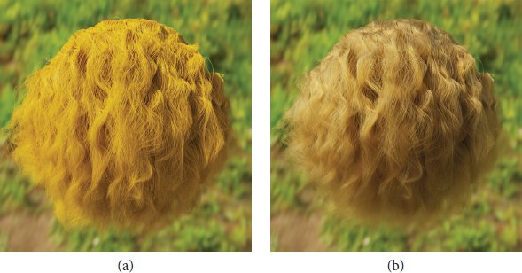
Figure 9.39: Comparison of a BSDF that Models Hair to a Coated Diffuse BSDF. (a) Geometric model of hair rendered using a BSDF based on a diffuse base layer with a rough dielectric interface above it (Section 14.3.3). (b) Model rendered using the HairBxDF from this section. Because the HairBxDF is based on an accurate model of the hair microgeometry and also models light transmission through hair, it gives a much more realistic appearance. (Hair geometry courtesy of Cem Yuksel.)
图 9.39:模拟头发的 BSDF 与涂层漫反射 BSDF 的比较。 (a) 使用基于漫射基层的 BSDF 渲染的头发几何模型,其上方有粗糙的介电界面(第 14.3.3 节)。 (b) 使用本节中的 HairBxDF 渲染的模型。由于 HairBxDF 基于头发微观几何的精确模型,并且还对通过头发的光传输进行建模,因此它提供了更加真实的外观。 (头发几何形状由 Cem Yuksel 提供。)
Curve 346
曲线346
DielectricBxDF 563
电介质BxDF 563
HairBxDF 606
头发BxDF 606
PiecewiseLinear2D 598
分段线性二维 598
Before discussing the mechanisms of light scattering from hair, we will start by defining a few ways of measuring incident and outgoing directions at ray intersection points on hair. In doing so, we will assume that the hair BSDF is used with the Curve shape from Section 6.7, which allows us to make assumptions about the parameterization of the hair geometry. For the geometric discussion in this section, we will assume that the Curve variant corresponding to a flat ribbon that is always facing the incident ray is being used. However, in the BSDF model, we will interpret intersection points as if they were on the surface of the corresponding swept cylinder. If there is no interpenetration between hairs and if the hair’s width is not much larger than a pixel’s width, there is no harm in switching between these interpretations.
在讨论头发光散射的机制之前,我们首先定义几种测量头发上光线交点处的入射和出射方向的方法。在此过程中,我们将假设头发 BSDF 与第 6.7 节中的曲线形状一起使用,这使我们能够对头发几何形状的参数化做出假设。对于本节中的几何讨论,我们将假设使用与始终面向入射光线的扁平带相对应的曲线变体。然而,在 BSDF 模型中,我们将解释交点,就好像它们位于相应扫掠圆柱体的表面上一样。如果毛发之间没有相互渗透,并且毛发的宽度不比像素的宽度大很多,那么在这些解释之间切换没有什么坏处。
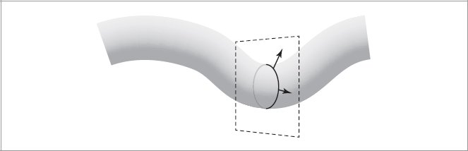
Figure 9.40: At any parametric point along a Curve shape, the cross-section of the curve is defined by a circle. All of the circle’s surface normals (arrows) lie in a plane (dashed lines), dubbed the “normal plane.”
图 9.40:在曲线形状上的任何参数点处,曲线的横截面由圆定义。圆的所有表面法线(箭头)都位于一个平面(虚线)内,称为“法线平面”。
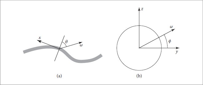
Figure 9.41: (a) Given a direction ω at a point on a curve, the longitudinal angle θ is defined by the angle between ω and the normal plane at the point (thick line). The curve’s tangent vector at the point is aligned with the x axis in the BSDF coordinate system. (b) For a direction ω, the azimuthal angle ϕ is found by projecting the direction into the normal plane and computing its angle with the y axis, which corresponds to the curve’s ∂p/∂v in the BSDF coordinate system.
图 9.41:(a) 给定曲线上某点的方向 ω,纵向角度 θ 由 ω 与该点处的法线平面(粗线)之间的角度定义。曲线在该点的切向量与 BSDF 坐标系中的 x 轴对齐。 (b) 对于方向 ω,通过将方向投影到法平面并计算其与 y 轴的角度来找到方位角 phi,该角度对应于 BSDF 坐标系中曲线的 ∂p/∂v。
Throughout the implementation of this scattering model, we will find it useful to separately consider scattering in the longitudinal plane, effectively using a side view of the curve, and scattering in the azimuthal plane, considering the curve head-on at a particular point along it. To understand these parameterizations, first recall that Curves are parameterized such that the u direction is along the length of the curve and v spans its width. At a given u, all the possible surface normals of the curve are given by the surface normals of the circular cross-section at that point. All of these normals lie in a plane that is called the normal plane (Figure 9.40).
在该散射模型的整个实现过程中,我们会发现单独考虑纵向平面中的散射(有效地使用曲线的侧视图)和方位角平面中的散射(考虑沿其特定点正面的曲线)是有用的。要理解这些参数化,首先回想一下曲线的参数化,使得 u 方向沿着曲线的长度,v 跨越其宽度。在给定 u 处,曲线的所有可能的表面法线均由该点处的圆形横截面的表面法线给出。所有这些法线都位于一个称为法线平面的平面上(图 9.40)。
We will find it useful to represent directions at a ray–curve intersection point with respect to coordinates (θ, ϕ) that are defined with respect to the normal plane at the u position where the ray intersected the curve. The angle θ is the longitudinal angle, which is the offset of the ray with respect to the normal plane (Figure 9.41(a)); θ ranges from −π/2 to π/2, where π/2 corresponds to a direction aligned with ∂p/∂u and −π/2 corresponds to −∂p/∂u. As explained in Section 9.1.1, in pbrt’s regular BSDF coordinate system, ∂p/∂u is aligned with the +x axis, so given a direction in the BSDF coordinate system, we have sin θ = ωx, since the normal plane is perpendicular to ∂p/∂u.
我们会发现,用坐标 (θ, phi) 表示射线与曲线交点处的方向很有用,该坐标是相对于射线与曲线相交的 u 位置处的法线平面定义的。角度θ为纵向角,即射线相对于法平面的偏移量(图9.41(a)); θ的范围从-π/2到π/2,其中π/2对应于与∂p/∂u对齐的方向,-π/2对应于-∂p/∂u。如第 9.1.1 节中所述,在 pbrt 的常规 BSDF 坐标系中,∂p/∂u 与 +x 轴对齐,因此给定 BSDF 坐标系中的方向,我们有 sin θ = ω x ,因为法线平面垂直于 ∂p/∂u。
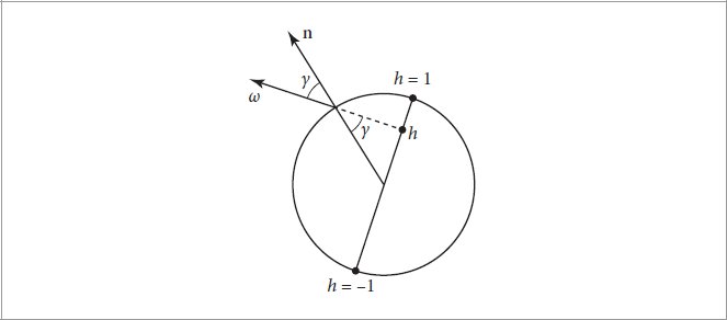
Figure 9.42: Given an incident direction ω of a ray that intersected a Curve projected to the normal plane, we can parameterize the curve’s width with h ∈ [−1, 1]. Given the h for a ray that has intersected the curve, trigonometry shows how to compute the angle γ between ω and the surface normal on the curve’s surface at the intersection point. The two angles γ are equal, and because the circle’s radius is 1, sin γ = h.
图 9.42:给定与投影到法线平面的曲线相交的光线的入射方向 ω,我们可以用 h ∈ [−1, 1] 参数化曲线的宽度。给定与曲线相交的射线的 h,三角学展示了如何计算 ω 与曲线表面交点处的表面法线之间的角度 γ。两个角度 γ 相等,由于圆的半径为 1,因此 sin γ = h。
In the BSDF coordinate system, the normal plane is spanned by the y and z coordinate axes. (y corresponds to ∂p/∂v for curves, which is always perpendicular to the curve’s ∂p/∂u, and z is aligned with the ribbon normal.) The azimuthal angle ϕ is found by projecting a direction ω into the normal plane and computing its angle with the y axis. It thus ranges from 0 to 2π (Figure 9.41(b)).
在 BSDF 坐标系中,法向平面由 y 和 z 坐标轴跨越。 (y 对应于曲线的 ∂p/∂v,它始终垂直于曲线的 ∂p/∂u,并且 z 与带状法线对齐。)方位角 phi 通过将方向 ω 投影到法线平面中来找到并计算它与 y 轴的角度。因此它的范围是从 0 到 2π(图 9.41(b))。
One more measurement with respect to the curve will be useful in the following. Consider incident rays with some direction ω: at any given parametric u value, all such rays that intersect the curve can only possibly intersect one half of the circle swept along the curve (Figure 9.42). We will parameterize the circle’s diameter with the variable h, where h = ±1 corresponds to the ray grazing the edge of the circle, and h = 0 corresponds to hitting it edge-on. Because pbrt parameterizes curves with v ∈ [0, 1] across the curve, we can compute h = −1 + 2v.
关于曲线的另一项测量将在下文中有用。考虑具有某个方向 ω 的入射光线:在任何给定的参数 u 值下,与曲线相交的所有此类光线仅可能与沿曲线扫过的圆的一半相交(图 9.42)。我们将用变量 h 参数化圆的直径,其中 h = ±1 对应于射线掠过圆的边缘,h = 0 对应于从边缘击中圆。因为 pbrt 将曲线参数化为 v ∈ [0, 1] 穿过曲线,所以我们可以计算 h = −1 + 2v。
Given the h for a ray intersection, we can compute the angle between the surface normal of the inferred swept cylinder (which is by definition in the normal plane) and the direction ω, which we will denote by γ. (Note: this is unrelated to the γn notation used for floating-point error bounds in Section 6.8.) See Figure 9.42, which shows that sin γ = h.
给定射线相交的 h,我们可以计算推断的扫掠圆柱体的表面法线(根据法线平面的定义)与方向 ω(我们将其表示为 γ)之间的角度。 (注:这与第 6.8 节中用于浮点误差界限的 γ n 表示法无关。)参见图 9.42,其中显示了 sin γ = h。
9.9.2 SCATTERING FROM HAIR
9.9.2 头发散射
Geometric setting in hand, we will now turn to discuss the general scattering behaviors that give hair its distinctive appearance and some of the assumptions that we will make in the following.
掌握了几何设置后,我们现在将讨论赋予头发独特外观的一般散射行为以及我们将在下面做出的一些假设。
Curve 346
曲线346
Hair and fur have three main components:
头发和毛皮由三个主要组成部分组成:
- Cuticle: The outer layer, which forms the boundary with air. The cuticle’s surface is a nested series of scales at a slight angle to the hair surface.
角质层:外层,与空气形成边界。角质层的表面是一系列嵌套的鳞片,与头发表面呈微小角度。 - Cortex: The next layer inside the cuticle. The cortex generally accounts for around 90% of hair’s volume but less for fur. It is typically colored with pigments that mostly absorb light.
皮质:角质层内的下一层。皮质通常占头发体积的 90% 左右,但皮毛的体积较少。它通常用主要吸收光的颜料着色。 - Medulla: The center core at the middle of the cortex. It is larger and more significant in thicker hair and fur. The medulla is also pigmented. Scattering from the medulla is much more significant than scattering from the medium in the cortex.
髓质:位于皮质中部的中心核心。它在较厚的毛发和毛皮中更大且更显着。髓质也有色素。来自髓质的散射比来自皮质中介质的散射更显着。
For the following scattering model, we will make a few assumptions. (Approaches for relaxing some of them are discussed in the exercises at the end of this chapter.) First, we assume that the cuticle can be modeled as a rough dielectric cylinder with scales that are all angled at the same angle α (effectively giving a nested series of cones; see Figure 9.43). We also treat the hair interior as a homogeneous medium that only absorbs light—scattering inside the hair is not modeled directly. (Chapters 11 and 14 have detailed discussion of light transport in participating media.)
对于下面的散射模型,我们将做出一些假设。 (本章末尾的练习中讨论了放松其中一些的方法。)首先,我们假设角质层可以建模为一个粗糙的介电圆柱体,其鳞片都以相同的角度 α 倾斜(有效地给出一系列嵌套的锥体;见图 9.43)。我们还将头发内部视为仅吸收光的均匀介质,头发内部的散射不会直接建模。 (第 11 章和第 14 章详细讨论了参与媒体中的光传输。)
We will also make the assumption that scattering can be modeled accurately by a BSDF—we model light as entering and exiting the hair at the same place. (A BSSRDF could certainly be used instead; the “Further Reading” section has pointers to work that has investigated that alternative.) Note that this assumption requires that the hair’s diameter be fairly small with respect to how quickly illumination changes over the surface; this assumption is generally fine in practice at typical viewing distances.
我们还将假设散射可以通过 BSDF 精确建模——我们将光建模为在同一位置进入和离开头发。 (当然可以使用 BSSRDF 来代替;“进一步阅读”部分提供了研究该替代方案的工作的指针。)请注意,此假设要求头发的直径相对于表面上的照明变化速度相当小;在典型的观看距离下,这种假设在实践中通常是正确的。
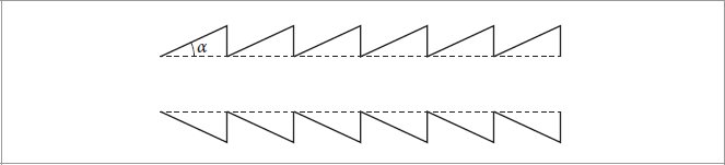
Figure 9.43: The surface of hair is formed by scales that deviate by a small angle α from the ideal cylinder. (α is generally around 2 − 4°; the angle shown here is larger for illustrative purposes.)
图 9.43:头发的表面由与理想圆柱体相差小角度 α 的鳞片形成。 (α 通常约为 2 – 4°;出于说明目的,此处显示的角度较大。)
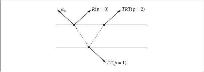
Figure 9.44: Incident light arriving at a hair can be scattered in a variety of ways. p = 0 corresponds to light reflected from the surface of the cuticle. Light may also be transmitted through the hair and leave the other side: p = 1. It may be transmitted into the hair and reflected back into it again before being transmitted back out: p = 2, and so forth.
图 9.44:到达头发的入射光可以通过多种方式进行散射。 p = 0 对应于从角质层表面反射的光。光也可以传输穿过头发并离开另一侧:p = 1。它可以传输到头发中并再次反射回头发中,然后再传输回来:p = 2,依此类推。
Incident light arriving at a hair may be scattered one or more times before leaving the hair; Figure 9.44 shows a few of the possible cases. We will use p to denote the number of path segments it follows inside the hair before being scattered back out to air. We will sometimes refer to terms with a shorthand that describes the corresponding scattering events at the boundary: p = 0 corresponds to R, for reflection, p = 1 is T T, for two transmissions p = 2 is TRT, p = 3 is TRRT, and so forth.
到达毛发的入射光在离开毛发之前可能会被散射一次或多次;图 9.44 显示了一些可能的情况。我们将使用 p 来表示头发在散回空气中之前所遵循的路径段数。我们有时会使用描述边界处相应散射事件的简写术语:p = 0 对应于 R,对于反射,p = 1 是 T T,对于两次传输 p = 2 是 TRT,p = 3 是 TRRT,等等。
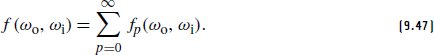
In the following, we will find it useful to consider these scattering modes separately and so will write the hair BSDF as a sum over terms p:
在下文中,我们会发现单独考虑这些散射模式很有用,因此将头发 BSDF 写为 p 项的总和:
To make the scattering model evaluation and sampling easier, many hair scattering models factor f into terms where one depends only on the angles θ and another on ϕ, the difference between ϕo and ϕi. This semi-separable model is given by:
为了使散射模型评估和采样更容易,许多头发散射模型将 f 分解为一些项,其中一个仅取决于角度 θ,另一个取决于 phi,即 phi o 和 phi 之间的差值。该半可分离模型由下式给出:

where we have a longitudinal scattering function Mp, an attenuation function Ap, and an azimuthal scattering function Np.7 The division by |cos θi| cancels out the corresponding factor in the reflection equation.
其中我们有一个纵向散射函数 M p 、一个衰减函数 A p 和一个方位角散射函数 N p 。 7 除以 |cos θ|抵消反射方程中的相应因子。
In the following implementation, we will evaluate the first few terms of the sum in Equation (9.47) and then represent all higher-order terms with a single one. The pMax constant controls how many are evaluated before the switch-over.
在下面的实现中,我们将评估方程(9.47)中总和的前几项,然后用单个项表示所有高阶项。 pMax 常数控制在切换之前评估的数量。
〈HairBxDF Constants〉 ≡ static constexpr int pMax = 3; |
606 |
The model implemented in the HairBxDF is parameterized by six values:
HairBxDF 中实现的模型由六个值参数化:
- h: the [−1, 1] offset along the curve width where the ray intersected the oriented ribbon.
h:沿着光线与定向带相交的曲线宽度的 [−1, 1] 偏移量。 - eta: the index of refraction of the interior of the hair (typically, 1.55).
eta:头发内部的折射率(通常为 1.55)。 - sigma_a: the absorption coefficient of the hair interior, where distance is measured with respect to the hair cylinder’s diameter. (The absorption coefficient is introduced in Section 11.1.1.)
sigma_a:头发内部的吸收系数,其中距离是相对于毛筒直径来测量的。 (吸收系数在11.1.1节中介绍。) - beta_m: the longitudinal roughness of the hair, mapped to the range [0, 1].
beta_m:头发的纵向粗糙度,映射到范围 [0, 1]。 - beta_n: the azimuthal roughness, also mapped to [0, 1].
beta_n:方位角粗糙度,也映射到 [0, 1]。 - alpha: the angle at which the small scales on the surface of hair are offset from the base cylinder, expressed in degrees (typically, 2).
alpha:头发表面的小鳞片偏离基础圆柱的角度,以度表示(通常为 2)。
〈HairBxDF Definition〉 ≡
〈HairBxDF 定义〉 ≡
class HairBxDF {
类 HairBxDF {
public:
民众:
〈HairBxDF Public Methods〉
〈HairBxDF 公共方法〉
private:
私人的:
〈HairBxDF Constants 606〉
〈HairBxDF常数606〉
〈HairBxDF Private Methods 608〉
〈HairBxDF 私有方法 608〉
〈HairBxDF Private Members 607〉
〈HairBxDF私人会员607〉
};
Beyond initializing corresponding member variables, the HairBxDF constructor performs some additional precomputation of values that will be useful for sampling and evaluation of the scattering model. The corresponding code will be added to the 〈HairBxDF constructor implementation〉 fragment in the following, closer to where the corresponding values are defined and used. Note that alpha is not stored in a member variable; it is used to compute a few derived quantities that will be, however.
除了初始化相应的成员变量之外,HairBxDF 构造函数还执行一些额外的值预计算,这对于散射模型的采样和评估非常有用。相应的代码将添加到下面的片段中,更靠近定义和使用相应值的地方。请注意,alpha 不存储在成员变量中;然而,它用于计算一些导出的量。
〈HairBxDF Private Members〉 ≡ Float h, eta; SampledSpectrum sigma_a; Float beta_m, beta_n; |
606 |
We will start with the method that evaluates the BSDF.
我们将从评估 BSDF 的方法开始。
〈HairBxDF Method Definitions〉 ≡
〈HairBxDF 方法定义〉 ≡
SampledSpectrum HairBxDF::f(Vector3f wo, Vector3f wi,
TransportMode mode) const {
TransportMode 模式) const {
〈Compute hair coordinate system terms related to wo 607〉
〈计算与wo 607相关的头发坐标系术语〉
〈Compute hair coordinate system terms related to wi 607〉
〈计算与wi 607相关的头发坐标系术语〉
〈Compute cos θt for refracted ray 610〉
〈计算折射光线 610 的 cos θ t 〉
〈Compute γt for refracted ray 610〉
〈计算折射光线610的γ t 〉
〈Compute the transmittance T of a single path through the cylinder 611〉
〈计算通过圆柱体611的单一路径的透过率T〉
〈Evaluate hair BSDF 616〉
〈评估头发 BSDF 616〉
}
There are a few quantities related to the directions ωo and ωi that are needed for evaluating the hair scattering model—specifically, the sine and cosine of the angle θ that each direction makes with the plane perpendicular to the curve, and the angle ϕ in the azimuthal coordinate system.
评估头发散射模型需要一些与方向 ω o 和 ω 相关的量,具体来说,每个方向与垂直于曲线的平面所成角度 θ 的正弦和余弦,以及方位坐标系中的角度 phi。
As explained in Section 9.9.1, sin θo is given by the x component of ωo in the BSDF coordinate system. Given sin θo, because θo ∈ [−π/2, π/2], we know that cos θo must be positive, and so we can compute cos θo using the identity sin2 θ + cos2 θ = 1. The angle ϕo in the perpendicular plane can be computed with std::atan.
如第 9.9.1 节中所述,sin θ o 由 BSDF 坐标系中 ω o 的 x 分量给出。给定 sin θ o ,因为 θ o ∈ [−π/2, π/2],我们知道 cos θ o 一定是正数,所以我们可以使用恒等式 sin 2 θ + cos 2 θ = 1 计算 cos θ o 。垂直方向上的角度 phi o 可以使用 std::atan 计算平面。
〈Compute hair coordinate system terms related to wo〉 ≡ Float sinTheta_o = wo.x; Float cosTheta_o = SafeSqrt(1 - Sqr(sinTheta_o)); Float phi_o = std::atan2(wo.z, wo.y); Float gamma_o = SafeASin(h); |
607, 619 |
Equivalent code computes these values for wi.
等效代码计算 wi 的这些值。
〈Compute hair coordinate system terms related to wi〉 ≡ Float sinTheta_i = wi.x; Float cosTheta_i = SafeSqrt(1 - Sqr(sinTheta_i)); Float phi_i = std::atan2(wi.z, wi.y); |
607 |
Float 23
浮法23
SafeASin() 1035
第1035章
SafeSqrt() 1034
第1034章
SampledSpectrum 171
采样频谱 171
Sqr() 1034
平方() 1034
TransportMode 571
运输方式 571
Vector3f 86
矢量3f 86
With these values available, we will consider in turn the factors of the BSDF model—Mp, Ap, and Np—before returning to the completion of the f() method.
有了这些值,我们将依次考虑 BSDF 模型的因素 - M p 、 A p 和 N p - 然后返回完成f() 方法的。
9.9.3 LONGITUDINAL SCATTERING
9.9.3 纵向散射
Mp defines the component of scattering related to the angles θ—longitudinal scattering. Longitudinal scattering is responsible for the specular lobe along the length of hair and the longitudinal roughness βm controls the size of this highlight. Figure 9.45 shows hair geometry rendered with three different longitudinal scattering roughnesses.
M p 定义与角度 θ 相关的散射分量——纵向散射。纵向散射负责沿着头发长度的镜面反射波瓣,纵向粗糙度 β m 控制该高光的大小。图 9.45 显示了用三种不同的纵向散射粗糙度渲染的头发几何形状。
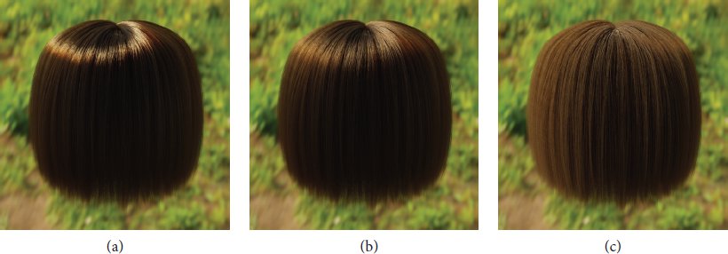
Figure 9.45: The Effect of Varying the Longitudinal Roughness βm. Hair model illuminated by a skylight environment map rendered with varying longitudinal roughness. (a) With a very low roughness, βm = 0.1, the hair appears too shiny—almost metallic. (b) With βm = 0.25, the highlight is similar to typical human hair. (c) At high roughness, βm = 0.7, the hair is unrealistically flat and diffuse. (Hair geometry courtesy of Cem Yuksel.)
图 9.45:改变纵向粗糙度 β m 的影响。由以不同纵向粗糙度渲染的天窗环境贴图照明的头发模型。 (a) 当粗糙度非常低时,β m = 0.1,头发显得太闪亮——几乎是金属的。 (b) 当 β m = 0.25 时,高光类似于典型的人类头发。 (c) 在高粗糙度下,β m = 0.7,毛发不切实际地平坦且分散。 (头发几何形状由 Cem Yuksel 提供。)
The mathematical details of the derivation of the scattering model are complex, so we will not include them here; as always, the “Further Reading” section has references to the details. The design goals of the model implemented here were that it be normalized (ensuring both energy conservation and no energy loss) and that it could be sampled directly. Although this model is not directly based on a physical model of how hair scatters light, it matches measured data well and has parametric control of roughness v.8
散射模型推导的数学细节很复杂,所以我们不会在这里包括它们;与往常一样,“进一步阅读”部分引用了详细信息。这里实现的模型的设计目标是标准化(确保能量守恒且无能量损失)并且可以直接采样。尽管该模型并非直接基于头发如何散射光的物理模型,但它与测量数据匹配良好,并且具有粗糙度 v 的参数控制。 8
The model is:
模型是:

where I0 is the modified Bessel function of the first kind and v is the roughness variance. Figure 9.46 shows plots of Mp.
其中 I 0 是第一类修正贝塞尔函数,v 是粗糙度方差。图 9.46 显示了 M p 的图。
This model is not numerically stable for low roughness variance values, so our implementation uses a different approach for that case that operates on the logarithm of I0 before taking an exponent at the end. The v <= .1 test in the implementation below selects between the two formulations.
对于低粗糙度方差值,该模型在数值上不稳定,因此我们的实现针对这种情况使用了不同的方法,即在最后取指数之前对 I 0 的对数进行运算。下面实现中的 v <= .1 测试在两个公式之间进行选择。
〈HairBxDF Private Methods〉 ≡ Float Mp(Float cosTheta_i, Float cosTheta_o, Float sinTheta_i, Float sinTheta_o, Float v) { Float a = cosTheta_i * cosTheta_o / v, b = sinTheta_i * sinTheta_o / v; Float mp = (v <= .1) ? (FastExp(LogI0(a) - b - 1 / v + 0.6931f + std::log(1 / (2 * v)))) : (FastExp(-b) * I0(a)) / (std::sinh(1 / v) * 2 * v); return mp; } |
606 |
FastExp() 1036
第1036章
Float 23
浮法23
I0() 1038
LogI0() 1038
第1038章
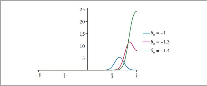
Figure 9.46: Plots of the Longitudinal Scattering Function. The shape of Mp as a function of θi for three values of θo. In all cases a roughness variance of v = 0.02 was used. The peaks are slightly shifted from the perfect specular reflection directions (at θi = 1, 1.3, and 1.4, respectively). (After d’Eon et al. (2011), Figure 4.)
图 9.46:纵向散射函数图。对于三个 θ o 值,M p 的形状作为 θ 的函数。在所有情况下,均使用 v = 0.02 的粗糙度方差。峰值稍微偏离完美镜面反射方向(分别在 θ = 1、1.3 和 1.4 处)。 (借鉴 d’Eon 等人 (2011),图 4。)
One challenge with this model is choosing a roughness v to achieve a desired look. Here we have implemented a perceptually uniform mapping from roughness βm ∈ [0, 1] to v where a roughness of 0 is nearly perfectly smooth and 1 is extremely rough. Different roughness values are used for different values of p. For p = 1, roughness is reduced by an empirical factor that models the focusing of light due to refraction through the circular boundary of the hair. It is then increased for p = 2 and subsequent terms, which models the effect of light spreading out after multiple reflections at the rough cylinder boundary in the interior of the hair.
该模型面临的一个挑战是选择粗糙度 v 以获得所需的外观。在这里,我们实现了从粗糙度 β m ε [0, 1] 到 v 的感知均匀映射,其中粗糙度 0 几乎完全平滑,1 则极其粗糙。不同的粗糙度值用于不同的 p 值。当 p = 1 时,粗糙度会因经验因子而降低,该因子模拟由于通过头发圆形边界的折射而导致的光聚焦。然后,当 p = 2 和后续项时,它会增加,从而模拟光在头发内部的粗糙圆柱边界处多次反射后扩散的效果。
〈HairBxDF constructor implementation〉 ≡ v[0] = Sqr(0.726f * beta_m + 0.812f * Sqr(beta_m) + 3.7f * Pow<20>(beta_m)); v[1] = .25 * v[0]; v[2] = 4 * v[0]; for (int p = 3; p <= pMax; ++p) v[p] = v[2]; |
|
〈HairBxDF Private Members〉 +≡ Float v[pMax + 1]; |
606 |
9.9.4 ABSORPTION IN FIBERS
9.9.4 纤维中的吸收
The Ap factor describes how the incident light is affected by each of the scattering modes p. It incorporates two effects: Fresnel reflection and transmission at the hair–air boundary and absorption of light that passes through the hair (for p > 0). Figure 9.47 has rendered images of hair with varying absorption coefficients, showing the effect of absorption. The Ap function that we have implemented models all reflection and transmission at the hair boundary as perfect specular—a very different assumption than Mp and Np (to come), which model glossy reflection and transmission. This assumption simplifies the implementation and gives reasonable results in practice (presumably in that the specular paths are, in a sense, averages over all the possible glossy paths).
A p 因子描述了每种散射模式 p 如何影响入射光。它包含两种效应:头发-空气边界处的菲涅耳反射和透射以及穿过头发的光的吸收(p > 0)。图 9.47 渲染了具有不同吸收系数的头发图像,显示了吸收的效果。我们实现的 A p 函数将头发边界处的所有反射和透射建模为完美镜面反射,这是与 M p 和 N p 非常不同的假设(即将推出),它模拟光泽反射和透射。这种假设简化了实现,并在实践中给出了合理的结果(大概是镜面反射路径在某种意义上是所有可能的光泽路径的平均值)。
We will start by finding the fraction of incident light that remains after a path of a single transmitted segment through the hair. To do so, we need to find the distance the ray travels until it exits the cylinder; the easiest way to do this is to compute the distances in the longitudinal and azimuthal projections separately.
我们将首先找到在穿过头发的单个透射段的路径之后剩余的入射光的分数。为此,我们需要找到光线离开圆柱体之前所经过的距离;最简单的方法是分别计算纵向和方位投影中的距离。
Float 23
浮法23
HairBxDF::beta_m 607
HairBxDF::pMax 606
头发BxDF::pMax 606
Pow() 1034
战俘() 1034
Sqr() 1034
平方() 1034
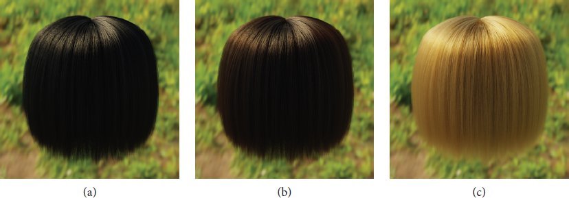
Figure 9.47: Hair Rendered with Various Absorption Coefficients. In all cases, βm = 0.25 and βn = 0.3. (a) σa = (3.35, 5.58, 10.96) (RGB coefficients): in black hair, almost all transmitted light is absorbed. The white specular highlight from the p = 0 term is the main visual feature. (b) σa = (0.84, 1.39, 2.74), giving brown hair, where the p > 1 terms all introduce color to the hair. (c) With a very low absorption coefficient of σa = (0.06, 0.10, 0.20), we have blonde hair. (Hair geometry courtesy of Cem Yuksel.)
图 9.47:使用不同吸收系数渲染的头发。在所有情况下,β m = 0.25 且 β n = 0.3。 (a) σ a = (3.35, 5.58, 10.96)(RGB 系数):在黑发中,几乎所有透射光都被吸收。 p = 0 项中的白色镜面高光是主要视觉特征。 (b) σ a = (0.84, 1.39, 2.74),给出棕色头发,其中 p > 1 项都为头发引入颜色。 (c) 吸收系数非常低 σ a = (0.06, 0.10, 0.20),我们的头发是金发。 (头发几何形状由 Cem Yuksel 提供。)
To compute these distances, we need the transmitted angles of the ray ωo, in the longitudinal and azimuthal planes, which we will denote by θt and γt, respectively. Application of Snell’s law using the hair’s index of refraction η allows us to compute sin θt and cos θt.
为了计算这些距离,我们需要射线 ω o 在纵向和方位平面中的透射角,我们将其表示为 θ t 和 γ t ,分别。应用斯涅耳定律并使用头发的折射率 η,我们可以计算 sin θ t 和 cos θ t 。
〈Compute cos θt for refracted ray〉 ≡ Float sinTheta_t = sinTheta_o / eta; Float cosTheta_t = SafeSqrt(1 - Sqr(sinTheta_t)); |
607, 618 |
For γt, although we could compute the transmitted direction ωt from ωo and then project ωt into the normal plane, it is possible to compute γt directly using a modified index of refraction that accounts for the effect of the longitudinal angle on the refracted direction in the normal plane. The modified index of refraction is given by
对于 γ t ,虽然我们可以根据 ω o 计算发射方向 ω t ,然后将 ω t 投影到法线平面中,可以使用修正的折射率直接计算 γ t ,该折射率考虑了纵向角度对法线平面中折射方向的影响。修改后的折射率由下式给出
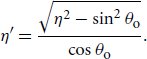
Given η′, we can compute the refracted direction γt directly in the normal plane.9 Since h = sin γo, we can apply Snell’s law to compute γt.
给定 η′,我们可以直接在法平面上计算折射方向 γ t 。 9 由于 h = sin γ o ,我们可以应用斯涅尔定律来计算 γ t 。
〈Compute γt for refracted ray〉 ≡ Float etap = SafeSqrt(Sqr(eta) - Sqr(sinTheta_o)) / cosTheta_o; Float sinGamma_t = h / etap; Float cosGamma_t = SafeSqrt(1 - Sqr(sinGamma_t)); Float gamma_t = SafeASin(sinGamma_t); |
607, 618, 619 |
If we consider the azimuthal projection of the transmitted ray in the normal plane, we can see that the segment makes the same angle γt with the circle normal at both of its endpoints (Figure 9.48). If we denote the total length of the segment by la, then basic trigonometry tells us that la/2 = cos γt, assuming a unit radius circle.
如果我们考虑透射光线在法线平面上的方位角投影,我们可以看到该线段在其两个端点处与圆法线形成相同的角度 γ t (图 9.48)。如果我们用 l a 表示线段的总长度,那么基本三角学告诉我们 l a /2 = cos γ t ,假设单位半径圆圈。
Float 23
浮法23
HairBxDF::eta 607
头发BxDF::eta 607
HairBxDF::h 607
头发BxDF::h 607
SafeASin() 1035
第1035章
SafeSqrt() 1034
第1034章
Sqr() 1034
平方() 1034
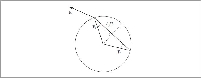
Figure 9.48: Computing the Transmitted Segment’s Distance. For a transmitted ray with angle γt with respect to the circle’s surface normal, half of the total distance la is given by cos γ, assuming a unit radius. Because γt is the same at both halves of the segment, la = 2 cos γt.
图 9.48:计算传输段的距离。对于相对于圆表面法线具有角度 γ t 的透射射线,总距离 l a 的一半由 cos γ 给出(假设单位半径)。由于 γ t 在该段的两半处相同,因此 l a = 2 cos γ t 。

Figure 9.49: The Effect of θt on the Transmitted Segment’s Length. The length of the transmitted segment through the cylinder is increased by a factor of 1/ cos θt versus a direct vertical path.
图 9.49:θ t 对传输段长度的影响。与直接垂直路径相比,通过圆柱体的传输段的长度增加了 1/ cos θ t 倍。
Now considering the longitudinal projection, we can see that the distance that a transmitted ray travels before exiting is scaled by a factor of 1/ cos θt as it passes through the cylinder (Figure 9.49). Putting these together, the total segment length in terms of the hair diameter is
现在考虑纵向投影,我们可以看到,透射光线在退出之前传播的距离在穿过圆柱体时按 1/ cos θ t 缩放(图 9.49)。将它们放在一起,以头发直径表示的总长度为

Given the segment length and the medium’s absorption coefficient, the fraction of light transmitted can be computed using Beer’s law, which is introduced in Section 11.2. Because the HairBxDF defined σa to be measured with respect to the hair diameter (so that adjusting the hair geometry’s width does not completely change its color), we do not consider the hair cylinder diameter when we apply Beer’s law, and the fraction of light remaining at the end of the segment is given by
给定线段长度和介质的吸收系数,可以使用第 11.2 节中介绍的比尔定律计算透射光的比例。由于 HairBxDF 定义 σ a 是相对于头发直径来测量的(因此调整头发几何形状的宽度不会完全改变其颜色),因此在应用比尔定律时,我们不考虑毛柱直径,段末端剩余的光分数由下式给出

〈Compute the transmittance T of a single path through the cylinder〉 ≡ SampledSpectrum T = Exp(-sigma_a * (2 * cosGamma_t / cosTheta_t)); |
607, 618 |
Given a single segment’s transmittance, we can now describe the function that evaluates the full Ap function. Ap() returns an array with the values of Ap up to pmax and a final value that is the sum of attenuations for all the higher-order scattering terms.
给定单个段的透射率,我们现在可以描述评估完整 A p 函数的函数。 Ap() 返回一个数组,其中包含 A p 到 p max 的值以及所有高阶散射项的衰减总和的最终值。
HairBxDF::sigma_a 607
头发BxDF::sigma_a 607
SampledSpectrum 171
采样频谱 171
SampledSpectrum::Exp() 172
采样频谱::Exp() 172
〈HairBxDF Private Methods〉 +≡ pstd::array<SampledSpectrum, pMax + 1> Ap(Float cosTheta_o, Float eta, Float h, SampledSpectrum T) { pstd::array<SampledSpectrum, pMax + 1> ap; 〈Compute p = 0 attenuation at initial cylinder intersection 612〉 〈Compute p = 1 attenuation term 612〉 〈Compute attenuation terms up to p = pMax 613〉 〈Compute attenuation term accounting for remaining orders of scattering 613〉 return ap; } |
606 |
For the A0 term, corresponding to light that reflects at the cuticle, the Fresnel reflectance at the air–hair boundary gives the fraction of light that is reflected. We can find the cosine of the angle between the surface normal and the direction vector with angles θo and γo in the hair coordinate system by cos θo cos γo.
对于 A 0 项,对应于在角质层反射的光,空气-头发边界处的菲涅耳反射率给出了反射光的比例。我们可以通过 cos θ o 求头发坐标系中角度为 θ o 和 γ o 的表面法线与方向向量之间夹角的余弦余弦γ o 。
〈Compute p = 0 attenuation at initial cylinder intersection〉 ≡ Float cosGamma_o = SafeSqrt(1 - Sqr(h)); Float cosTheta = cosTheta_o * cosGamma_o; Float f = FrDielectric(cosTheta, eta); ap[0] = SampledSpectrum(f); |
612 |
For the T T term, p = 1, we have two 1 − f factors, accounting for transmission into and out of the cuticle boundary, and a single T factor for one transmission path through the hair.
对于 T T 项,p = 1,我们有两个 1 − f 因子,用于考虑进出角质层边界的传输,以及一个用于通过头发的一条传输路径的 T 因子。
〈Compute p = 1 attenuation term〉 ≡ ap[1] = Sqr(1 - f) * T; |
612 |
The p = 2 term has one more reflection event, reflecting light back into the hair, and then a second transmission term. Since we assume perfect specular reflection at the cuticle boundary, both segments inside the hair make the same angle γt with the circle’s normal (Figure 9.50). From this, we can see that both segments must have the same length (and so forth for subsequent segments). In general, for p > 0,
p = 2 项还有一个反射事件,将光反射回头发,然后是第二个透射项。由于我们假设角质层边界处存在完美的镜面反射,因此头发内部的两个部分与圆的法线形成相同的角度 γ t (图 9.50)。由此,我们可以看到两个段必须具有相同的长度(后续段依此类推)。一般来说,当 p > 0 时,
Ap = Ap−1T f = (1 − f )2Tp f p−1.
A p = A p−1 T f = (1 − f ) 2 T p f p−1 。
Float 23
浮法23
FrDielectric() 557
HairBxDF::eta 607
头发BxDF::eta 607
HairBxDF::h 607
头发BxDF::h 607
HairBxDF::pMax 606
头发BxDF::pMax 606
SafeSqrt() 1034
第1034章
SampledSpectrum 171
采样频谱 171
Sqr() 1034
平方() 1034
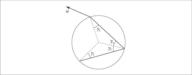
Figure 9.50: When a transmitted ray undergoes specular reflection at the interior of the hair cylinder, it makes the same angle γt with the circle’s surface normal as the original transmitted ray did. From this, it follows that the lengths of all ray segments for a path inside the cylinder must be equal.
图 9.50:当透射光线在毛筒内部进行镜面反射时,它与圆的表面法线形成与原始透射光线相同的角度 γ t 。由此可见,圆柱体内路径的所有光线段的长度必须相等。
〈Compute attenuation terms up to p = pMax〉 ≡ for (int p = 2; p < pMax; ++p) ap[p] = ap[p - 1] * T * f; |
612 |
After pMax, a final term accounts for all further orders of scattering. The sum of the infinite series of remaining terms can fortunately be found in closed form, since both T < 1 and f < 1:
在 pMax 之后,最后一项解释了所有进一步的散射阶数。幸运的是,剩余项的无限级数的总和可以以封闭形式找到,因为 T < 1 且 f < 1:
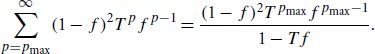
〈Compute attenuation term accounting for remaining orders of scattering〉 ≡ if (1 - T * f) ap[pMax] = ap[pMax - 1] * f * T / (1 - T * f); |
612 |
9.9.5 AZIMUTHAL SCATTERING
9.9.5 方位角散射
Finally, we will model the component of scattering dependent on the angle ϕ. We will do this work entirely in the normal plane. The azimuthal scattering model is based on first computing a new azimuthal direction assuming perfect specular reflection and transmission and then defining a distribution of directions around this central direction, where increasing roughness gives a wider distribution. Therefore, we will first consider how an incident ray is deflected by specular reflection and transmission in the normal plane; Figure 9.51 illustrates the cases for the first two values of p.
最后,我们将对取决于角度 的散射分量进行建模。我们将完全在法线平面上完成这项工作。方位角散射模型首先计算假设完美镜面反射和透射的新方位角方向,然后定义围绕该中心方向的方向分布,其中增加粗糙度会产生更宽的分布。因此,我们首先考虑入射光线如何在法平面内通过镜面反射和透射而发生偏转;图 9.51 说明了 p 前两个值的情况。
Following the reasoning from Figure 9.51, we can derive the function Φ, which gives the net change in azimuthal direction:
按照图 9.51 的推理,我们可以推导出函数 Φ,它给出了方位角方向的净变化:
Φ(p, h) = 2pγt − 2γo + pπ.
Φ(p, h) = 2pγ t − 2γ o + pπ。
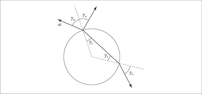
Figure 9.51: For specular reflection, with p = 0, the incident and reflected directions make the same angle γo with the surface normal. The net change in angle is thus −2γo. For p = 1, the ray is deflected from γo to γt when it enters the cylinder and then correspondingly on the way out. We can also see that when the ray is transmitted again out of the circle, it makes an angle γo with the surface normal there. Adding up the angles, the net deflection is 2γt − 2γo + π.
图 9.51:对于镜面反射,当 p = 0 时,入射方向和反射方向与表面法线形成相同的角度 γ o 。因此,角度的净变化为 -2γ o 。当 p = 1 时,光线在进入圆柱体时从 γ o 偏转到 γ t ,然后在离开圆柱体时相应地偏转 γ t 。我们还可以看到,当光线再次传输到圆外时,它与圆处的表面法线形成角度 γ o 。将角度相加,净偏转为 2γ t − 2γ o + π。
HairBxDF::pMax 606
头发BxDF::pMax 606
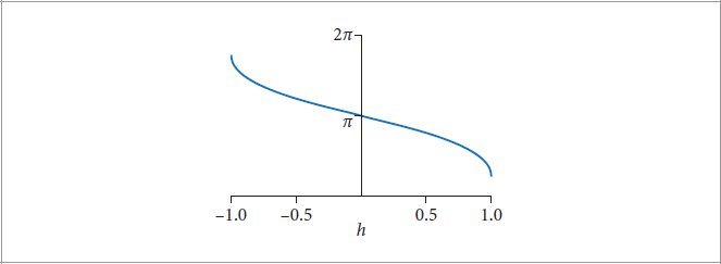
Figure 9.52: Plot of Φ(p, h) for p = 1. As h varies from −1 to 1, we can see that the range of orientations ϕ for the specularly transmitted ray varies rapidly. By examining the range of ϕ values, we can see that the possible transmitted directions cover roughly 2/3 of all possible directions on the circle.
图 9.52:p = 1 时的 Φ(p, h) 绘图。当 h 从 -1 变化到 1 时,我们可以看到镜面透射光线的方向范围 phi 变化很快。通过检查 ψ 值的范围,我们可以看到可能的传输方向大约覆盖圆上所有可能方向的 2/3。
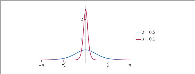
Figure 9.53: Plots of the Trimmed Logistic Function over ±π. The curve for s = 0.5 (blue line) is broad and flat, while at s = 0.1 (red line), the curve is peaked. Because the function is normalized, the peak at 0 generally does not have the value 1, unlike the Gaussian.
图 9.53:修剪 Logistic 函数在 ±π 上的图。 s = 0.5(蓝线)时的曲线宽且平坦,而 s = 0.1(红线)时,曲线出现峰值。由于函数已归一化,因此与高斯函数不同,0 处的峰值通常不具有值 1。
(Recall that γo and γt are derived from h.) Figure 9.52 shows a plot of this function for p = 1.
(回想一下 γ o 和 γ t 是从 h 导出的。)图 9.52 显示了 p = 1 时该函数的图。
〈HairBxDF Private Methods〉 +≡ Float Phi(int p, Float gamma_o, Float gamma_t) { return 2 * p * gamma_t - 2 * gamma_o + p * Pi; } |
606 |
Now that we know how to compute new angles in the normal plane after specular transmission and reflection, we need a way to represent surface roughness, so that a range of directions centered around the specular direction can contribute to scattering. The logistic distribution provides a good option: it is a generally useful one for rendering, since it has a similar shape to the Gaussian, while also being normalized and integrable in closed form (unlike the Gaussian); see Section B.2.5 for more information.
现在我们知道如何计算镜面透射和反射后法线平面中的新角度,我们需要一种表示表面粗糙度的方法,以便以镜面方向为中心的一系列方向可以有助于散射。逻辑分布提供了一个很好的选择:它对于渲染通常有用,因为它具有与高斯分布相似的形状,同时也可以以封闭形式标准化和可积(与高斯分布不同);有关详细信息,请参阅第 B.2.5 节。
In the following, we will find it useful to define a normalized logistic function over a range [a, b]; we will call this the trimmed logistic, lt.
在下文中,我们将发现在范围 [a, b] 上定义归一化逻辑函数非常有用;我们将其称为修剪逻辑, l t 。
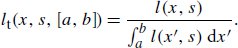
Float 23
浮法23
Pi 1033
圆周率1033
Figure 9.53 shows plots of the trimmed logistic distribution for a few values of s.
图 9.53 显示了几个 s 值的修剪逻辑分布图。
Now we have the pieces to be able to implement the azimuthal scattering distribution. The Np() function computes the Np term, finding the angular difference between ϕ and Φ(p, h) and evaluating the azimuthal distribution with that angle.
现在我们有了能够实现方位角散射分布的部件。 Np() 函数计算 N p 项,找出 phi 和 Φ(p, h) 之间的角度差,并用该角度评估方位角分布。
〈HairBxDF Private Methods〉 +≡ Float Np(Float phi, int p, Float s, Float gamma_o, Float gamma_t) { Float dphi = phi - Phi(p, gamma_o, gamma_t); 〈Remap dphi to [−π, π] 615〉 return TrimmedLogistic(dphi, s, -Pi, Pi); } |
606 |
The difference between ϕ and Φ(p, h) may be outside the range we have defined the logistic over, [−π, π], so we rotate around the circle as needed to get the value to the right range. Because dphi never gets too far out of range for the small p used here, we use the simple approach of adding or subtracting 2π as needed.
Φ 和 Φ(p, h) 之间的差异可能超出我们定义的逻辑分布 [−π, π] 的范围,因此我们根据需要绕圆旋转以使值达到正确的范围。由于 dphi 永远不会超出此处使用的小 p 的范围太远,因此我们使用根据需要添加或减去 2π 的简单方法。
〈Remap dphi to [−π, π]〉 ≡ while (dphi > Pi) dphi -= 2 * Pi; while (dphi < -Pi) dphi += 2 * Pi; |
615 |
As with the longitudinal roughness, it is helpful to have a roughly perceptually linear mapping from azimuthal roughness βn ∈ [0, 1] to the logistic scale factor s.
与纵向粗糙度一样,从方位粗糙度 β n ε [0, 1] 到逻辑比例因子 s 的大致感知线性映射是有帮助的。
〈HairBxDF constructor implementation〉 +≡ static const Float SqrtPiOver8 = 0.626657069f; s = SqrtPiOver8 * (0.265f * beta_n + 1.194f * Sqr(beta_n) + 5.372f * Pow<22>(beta_n)); |
|
〈HairBxDF Private Members〉 +≡ Float s; |
606 |
Figure 9.54 shows polar plots of azimuthal scattering for the T T term, p = 1, with a fairly low roughness. The scattering distributions for the two different points on the curve’s width are quite different. Because we expect the hair width to be roughly pixel-sized, many rays per pixel are needed to resolve this variation well.
图 9.54 显示了 T T 项 p = 1 的方位角散射的极坐标图,粗糙度相当低。曲线宽度上两个不同点的散射分布有很大不同。因为我们预计头发宽度大致为像素大小,所以每个像素需要许多光线才能很好地解决这种变化。
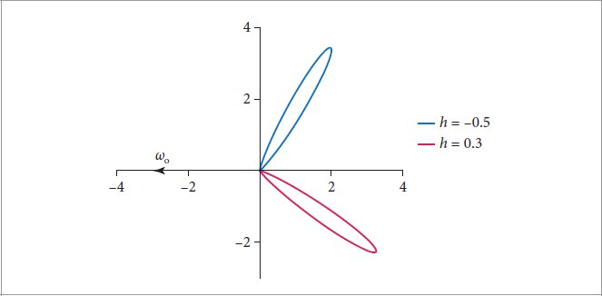
Figure 9.54: Polar plots of Np for p = 1, θo aligned with the −x axis, and with a low roughness, βn = 0.1, for (blue) h = −0.5 and (red) h = 0.3. We can see that Np varies rapidly over the width of the hair.
图 9.54:p = 1、θ o 与 -x 轴对齐且粗糙度较低、β n = 0.1 时 N p 的极坐标图,对于(蓝色)h = −0.5 和(红色)h = 0.3。我们可以看到 N p 在头发宽度上快速变化。
Float 23
浮法23
HairBxDF::beta_n 607
HairBxDF::Phi() 614
第614章
Pi 1033
圆周率1033
Pow() 1034
战俘() 1034
Sqr() 1034
平方() 1034
TrimmedLogistic() 1038
修剪物流() 1038
9.9.6 SCATTERING MODEL EVALUATION
9.9.6 散射模型评估
We now have almost all the pieces we need to be able to evaluate the model. The last detail is to account for the effect of scales on the hair surface (recall Figure 9.43). Suitable adjustments to θo work well to model this characteristic of hair.
我们现在几乎拥有了评估模型所需的所有部分。最后一个细节是考虑鳞片对头发表面的影响(回想图 9.43)。对 θ o 进行适当的调整可以很好地模拟头发的这种特征。
For the R term, adding the angle 2α to θo can model the effect of evaluating the hair scattering model with respect to the surface normal of a scale. We can then go ahead and evaluate M0 with this modification to θo. For T T, we have to account for two transmission events through scales. Rotating by α in the opposite direction approximately compensates. (Because the refraction angle is nonlinear with respect to changes in normal orientation, there is some error in this approximation, though the error is low for the typical case of small values of α.) TRT has a reflection term inside the hair; a rotation by −4α compensates for the overall effect.
对于R项,将角度2α添加到θ o 可以模拟评估毛发散射模型相对于鳞片表面法线的效果。然后我们可以通过对 θ o 的修改来继续评估 M 0 。对于 T T,我们必须通过尺度来解释两个传输事件。沿相反方向旋转 α 即可近似补偿。 (由于折射角相对于法向方向的变化是非线性的,因此该近似值存在一些误差,尽管对于小 α 值的典型情况误差很小。)TRT 在头发内部有一个反射项; -4α 的旋转可以补偿整体效果。
The effects of these shifts are that the primary reflection lobe R is offset to be above the perfect specular direction and the secondary TRT lobe is shifted below it. Together, these lead to two distinct specular highlights of different colors, since R is not affected by the hair’s color, while TRT picks up the hair color due to absorption. This effect can be seen in human hair and is evident in the images in Figure 9.45, for example.
这些偏移的影响是主反射波瓣 R 偏移到完美镜面反射方向上方,而辅助 TRT 波瓣偏移到其下方。这些共同导致了两种不同颜色的不同镜面高光,因为 R 不受头发颜色的影响,而 TRT 由于吸收而拾取头发颜色。这种效果可以在人类头发中看到,并且在图 9.45 中的图像中很明显。
Because we only need the sine and cosine of the angle θi to evaluate Mp, we can use the trigonometric identities
因为我们只需要角度 θ 的正弦和余弦来计算 M p ,所以我们可以使用三角恒等式
sin(θo ± α) = sin θo cos α ± cos θo sin α
cos(θo ± α) = cos θo cos α ∓ sin θo sin α
to efficiently compute the rotated angles without needing to evaluate any additional trigonometric functions. The HairBxDF constructor therefore precomputes sin(2kα) and cos(2kα) for k = 0, 1, 2. These values can be computed particularly efficiently using trigonometric double angle identities: cos 2θ = cos2 θ − sin2 θ and sin 2θ = 2 cos θ sin θ.
有效计算旋转角度,无需计算任何额外的三角函数。因此,HairBxDF 构造函数会预先计算 k = 0, 1, 2 时的 sin(2 k α) 和 cos(2 k α)。使用三角双角可以特别有效地计算这些值恒等式:cos 2θ = cos 2 θ − sin 2 θ 和 sin 2θ = 2 cos θ sin θ。
〈HairBxDF constructor implementation〉 +≡ sin2kAlpha[0] = std::sin(Radians(alpha)); cos2kAlpha[0] = SafeSqrt(1 - Sqr(sin2kAlpha[0])); for (int i = 1; i < pMax; ++i) { sin2kAlpha[i] = 2 * cos2kAlpha[i - 1] * sin2kAlpha[i - 1]; cos2kAlpha[i] = Sqr(cos2kAlpha[i - 1]) - Sqr(sin2kAlpha[i - 1]); } |
|
〈HairBxDF Private Members〉 +≡ Float sin2kAlpha[pMax], cos2kAlpha[pMax]; |
606 |
AbsCosTheta() 107
Float 23
浮法23
HairBxDF 606
头发BxDF 606
HairBxDF::Ap() 612
第612章
HairBxDF::eta 607
头发BxDF::eta 607
HairBxDF::h 607
头发BxDF::h 607
HairBxDF::Mp() 608
第608章
HairBxDF::Np() 615
第615章
HairBxDF::pMax 606
头发BxDF::pMax 606
HairBxDF::v 609
头发BxDF::v 609
Radians() 1033
弧度() 1033
SafeSqrt() 1034
第1034章
SampledSpectrum 171
采样频谱 171
Sqr() 1034
平方() 1034
Evaluating the model is now mostly just a matter of calling functions that have already been defined and summing the individual terms fp.
现在评估模型主要只是调用已定义的函数并对各个项 f p 求和。
The rotations that account for the effect of scales are implemented using the trigonometric identities listed above. Here is the code for the p = 0 case, where θo is rotated by 2α. The remaining cases follow the same structure. (The rotation is by −α for p = 1 and by −4α for p = 2.)
考虑比例效应的旋转是使用上面列出的三角恒等式来实现的。这是 p = 0 情况的代码,其中 θ o 旋转 2α。其余案例遵循相同的结构。 (对于 p = 1,旋转为 -α;对于 p = 2,旋转为 -4α。)
〈Compute sin θo and cos θo terms accounting for scales〉 ≡ Float sinThetap_o, cosThetap_o; if (p == 0) { sinThetap_o = sinTheta_o * cos2kAlpha[1] - cosTheta_o * sin2kAlpha[1]; cosThetap_o = cosTheta_o * cos2kAlpha[1] + sinTheta_o * sin2kAlpha[1]; } 〈Handle remainder of p values for hair scale tilt〉 〈Handle out-of-range cos θo from scale adjustment 617〉 |
616, 619, 620 |
When ωi is nearly parallel with the hair, the scale adjustment may give a slightly negative value for cos θi—effectively, in this case, it represents a θi that is slightly greater than π/2, the maximum expected value of θ in the hair coordinate system. This angle is equivalent to π − θi, and cos(π − θi) = |cos θi|, so we can easily handle that here.
当 ω 几乎与头发平行时,比例调整可能会给出 cos θ 的稍微负值 - 实际上,在这种情况下,它表示略大于 π/2(头发中 θ 的最大期望值)的 θ坐标系。这个角度相当于 π − θ,并且 cos(π − θ) = |cos θ|,所以我们在这里可以轻松处理。
〈Handle out-of-range cos θo from scale adjustment〉 ≡ cosThetap_o = std::abs(cosThetap_o); |
617, 620 |
A final term accounts for all higher-order scattering inside the hair. We just use a uniform distribution N(ϕ) = 1/(2π) for the azimuthal distribution; this is a reasonable choice, as the direction offsets from Φ(p, h) for p ≥ pmax generally have wide variation and the final Ap term generally represents less than 15% of the overall scattering, so little error is introduced in the final result.
最后一项解释了头发内部的所有高阶散射。我们仅使用均匀分布 N(phi) = 1/(2π) 来表示方位角分布;这是一个合理的选择,因为 p ≥ p max 时与 Φ(p, h) 的方向偏移通常具有很大的变化,并且最终的 A p 项通常表示小于 15%总体散射的影响,因此最终结果中引入的误差很小。
〈Compute contribution of remaining terms after pMax〉 ≡ fsum += Mp(cosTheta_i, cosTheta_o, sinTheta_i, sinTheta_o, v[pMax]) * ap[pMax] / (2 * Pi); |
616 |
A Note on Reciprocity
关于互惠的注释
Although we included reciprocity in the properties of physically valid BRDFs in Section 4.3.1, the model we have implemented in this section is, unfortunately, not reciprocal. An immediate issue is that the rotation for hair scales is applied only to θi. However, there are more problems: first, all terms p > 0 that involve transmission are not reciprocal since the transmission terms use values based on ωt, which itself only depends on ωo. Thus, if ωo and ωi are interchanged, a completely different ωt is computed, which in turn leads to different cos θt and γt values, which in turn give different values from the Ap and Np functions. In practice, however, we have not observed artifacts in images from these shortcomings.
尽管我们在第 4.3.1 节中将互易性纳入了物理上有效的 BRDF 的属性中,但不幸的是,我们在本节中实现的模型不是互易性的。一个迫在眉睫的问题是毛鳞片的旋转仅适用于 θ。然而,还有更多问题:首先,所有涉及传输的项 p > 0 都不是互易的,因为传输项使用基于 ω t 的值,而 ω t 本身仅取决于 ω o 。因此,如果 ω o 和 ω 互换,则会计算出完全不同的 ω t ,从而导致不同的 cos θ t 和 γ t 值,这又从 A p 和 N p 函数给出不同的值。然而,在实践中,我们还没有观察到这些缺陷造成的图像伪影。
AbsCosTheta() 107
Float 23
浮法23
HairBxDF::cos2kAlpha 616
头发BxDF::cos2kAlpha 616
HairBxDF::Mp() 608
第608章
HairBxDF::sin2kAlpha 616
头发BxDF::sin2kAlpha 616
Pi 1033
圆周率1033
Being able to generate sampled directions and compute the PDF for sampling a given direction according to a distribution that is similar to the overall BSDF is critical for efficient rendering, especially at low roughnesses, where the hair BSDF varies rapidly as a function of direction. In the approach implemented here, samples are generated with a two-step process: first we choose a p term to sample according to a probability based on each term’s Ap function value, which gives its contribution to the overall scattering function. Then, we find a direction by sampling the corresponding Mp and Np terms.10 Fortunately, both the Mp and Np terms of the hair BSDF can be sampled perfectly, leaving us with a sampling scheme that exactly matches the PDF of the full BSDF.
能够生成采样方向并根据类似于整体 BSDF 的分布计算给定方向采样的 PDF 对于高效渲染至关重要,尤其是在低粗糙度情况下,其中头发 BSDF 作为方向的函数快速变化。在这里实现的方法中,样本是通过两步过程生成的:首先,我们根据每个项的 A p 函数值的概率选择一个 p 项进行采样,该函数值给出了它对整体散射的贡献功能。然后,我们通过采样相应的 M p 和 N p 项来找到方向。 10 幸运的是,头发 BSDF 的 M p 和 N p 项都可以完美采样,为我们提供了与 PDF 完全匹配的采样方案完整的 BSDF。
We will first define the ApPDF() method, which returns a discrete PDF with probabilities for sampling each term Ap according to its contribution relative to all the Ap terms, given θo.
我们将首先定义 ApPDF() 方法,该方法返回一个离散 PDF,其中包含根据每个项 A p 相对于所有 A p 项的贡献对每个项 A p 进行采样的概率,给定 θ < b2> 。
〈HairBxDF Method Definitions〉 +≡
〈HairBxDF 方法定义〉 +≡
pstd::array<Float, HairBxDF::pMax + 1>
pstd::array<浮点,HairBxDF::pMax + 1>
HairBxDF::ApPDF(Float cosTheta_o) const {
〈Initialize array of Ap values for cosTheta_o 618〉
〈为 cosTheta_o 618 初始化 A p 值数组〉
〈Compute Ap PDF from individual Ap terms 618〉
〈根据单个 A p 项计算 A p PDF618〉
return apPDF;
返回appPDF;
}
The method starts by computing the values of Ap for cosTheta_o. We are able to reuse some previously defined fragments to make this task easier.
该方法首先计算 cosTheta_o 的 A p 值。我们能够重用一些先前定义的片段来使这项任务变得更容易。
〈Initialize array of Ap values for cosTheta_o〉 ≡ Float sinTheta_o = SafeSqrt(1 - Sqr(cosTheta_o)); 〈Compute cos θt for refracted ray 610〉 〈Compute γt for refracted ray 610〉 〈Compute the transmittance T of a single path through the cylinder 611〉 pstd::array<SampledSpectrum, pMax + 1> ap = Ap(cosTheta_o, eta, h, T); |
618 |
Next, the spectral Ap values are converted to scalars using their luminance and these values are normalized to make a proper PDF.
接下来,使用其亮度将光谱 A p 值转换为标量,并对这些值进行归一化以生成适当的 PDF。
〈Compute Ap PDF from individual Ap terms〉 ≡ pstd::array<Float, pMax + 1> apPDF; Float sumY = 0; for (const SampledSpectrum &as : ap) sumY += as.Average(); for (int i = 0; i <= pMax; ++i) apPDF[i] = ap[i].Average() / sumY; |
618 |
With these preliminaries out of the way, we can now implement the Sample_f() method.
完成这些准备工作后,我们现在可以实现 Sample_f() 方法。
Float 23
浮法23
HairBxDF::Ap() 612
第612章
HairBxDF::h 607
头发BxDF::h 607
HairBxDF::pMax 606
头发BxDF::pMax 606
SafeSqrt() 1034
第1034章
SampledSpectrum 171
采样频谱 171
SampledSpectrum::Average() 172
采样频谱::平均() 172
Sqr() 1034
平方() 1034
〈HairBxDF Method Definitions〉 +≡
〈HairBxDF 方法定义〉 +≡
pstd::optional<BSDFSample>
pstd::可选
HairBxDF::Sample_f(Vector3f wo, Float uc, Point2f u, TransportMode mode,
HairBxDF::Sample_f(Vector3f wo, Float uc, Point2f u, TransportMode 模式,
BxDFReflTransFlags sampleFlags) const {
〈Compute hair coordinate system terms related to wo 607〉
〈计算与wo 607相关的头发坐标系术语〉
〈Determine which term p to sample for hair scattering 619〉
〈确定毛发散射的样本 p 619〉
〈Compute sin θo and cos θo terms accounting for scales 617〉
〈计算考虑尺度的 sin θ o 和 cos θ o 项 617〉
〈Sample Mp to compute θi 619〉
〈样本 M p 计算 θ619〉
〈Sample Np to compute Δϕ 619〉
〈样本 N p 计算 Δψ 619〉
〈Compute wi from sampled hair scattering angles 620〉
〈根据采样的头发散射角度 620 计算 wi〉
〈Compute PDF for sampled hair scattering direction wi 620〉
〈计算 620 采样头发散射方向的 PDF〉
return BSDFSample(f(wo, wi, mode), wi, pdf, Flags());
返回 BSDFSample(f(wo, wi, 模式), wi, pdf, Flags());
}
Given the PDF over Ap terms, a call to SampleDiscrete() takes care of choosing one. Because we only need to generate one sample from the PDF’s distribution, the work to compute an explicit CDF array (for example, by using PiecewiseConstant1D) is not worthwhile. Note that we take advantage of SampleDiscrete()’s optional capability of returning a fresh uniform random sample, overwriting the value in uc. This sample value will be used shortly for sampling Np.
给定 A p 项上的 PDF,调用 SampleDiscrete() 负责选择一项。因为我们只需要从 PDF 分布中生成一个样本,所以计算显式 CDF 数组(例如,通过使用 PiecewiseConstant1D)的工作是不值得的。请注意,我们利用 SampleDiscrete() 的可选功能返回新鲜的均匀随机样本,覆盖 uc 中的值。该样本值很快将用于采样 N p 。
〈Determine which term p to sample for hair scattering〉 ≡ pstd::array<Float, pMax + 1> apPDF = ApPDF(cosTheta_o); int p = SampleDiscrete(apPDF, uc, nullptr, &uc); |
619 |
We can now sample the corresponding Mp term given θo to find θi. The derivation of this sampling method is fairly involved, so we will include neither the derivation nor the implementation here. This fragment, 〈Sample Mp to compute θi〉, consumes both of the sample values u[0] and u[1] and initializes variables sinTheta_i and cosTheta_i according to the sampled direction.
现在,我们可以对给定 θ o 的相应 M p 项进行采样来找到 θ。这种采样方法的推导相当复杂,因此我们在这里既不包括推导,也不包括实现。该片段 tocompute θ>,消耗样本值u[0]和u[1],并根据采样方向初始化变量sinTheta_i和cosTheta_i。
〈Sample Mp to compute θi〉 ≡ Float cosTheta = 1 + v[p] * std::log(std::max<Float>(u[0], 1e-5) + (1 - u[0]) * FastExp(-2 / v[p])); Float sinTheta = SafeSqrt(1 - Sqr(cosTheta)); Float cosPhi = std::cos(2 * Pi * u[1]); Float sinTheta_i = -cosTheta * sinThetap_o + sinTheta * cosPhi * cosThetap_o; Float cosTheta_i = SafeSqrt(1 - Sqr(sinTheta_i)); |
619 |
BSDFSample 541
BSDF样本 541
BxDF::Flags() 538
第538章
BxDFReflTransFlags 540
FastExp() 1036
第1036章
Float 23
浮法23
HairBxDF::ApPDF() 618
第618章
HairBxDF::f() 607
第607章
HairBxDF::Phi() 614
第614章
HairBxDF::pMax 606
头发BxDF::pMax 606
HairBxDF::v 609
头发BxDF::v 609
Pi 1033
圆周率1033
PiecewiseConstant1D 1009
分段常数1D 1009
Point2f 92
点2f 92
SafeSqrt() 1034
第1034章
SampleDiscrete() 70
样本离散() 70
SampleTrimmedLogistic() 1006
第1006章
SphericalDirection() 106
球面方向() 106
Sqr() 1034
平方() 1034
TransportMode 571
运输方式 571
Vector3f 86
矢量3f 86
Next we will sample the azimuthal distribution Np. For terms up to pmax, we take a sample from the logistic distribution centered around the exit direction given by Φ(p, h). For the last term, we sample from a uniform distribution.
接下来我们将对方位分布 N p 进行采样。对于 p max 之前的项,我们从以 Φ(p, h) 给出的退出方向为中心的逻辑分布中抽取样本。对于最后一项,我们从均匀分布中采样。
〈Sample Np to compute Δϕ〉 ≡ 〈Compute γt for refracted ray 610〉 Float dphi; if (p < pMax) dphi = Phi(p, gamma_o, gamma_t) + SampleTrimmedLogistic(uc, s, -Pi, Pi); else dphi = 2 * Pi * uc; |
619 |
Given θi and ϕi, we can compute the sampled direction wi. The math is similar to that used in the SphericalDirection() function, but with two important differences. First, because here θ is measured with respect to the plane perpendicular to the cylinder rather than the cylinder axis, we need to compute cos(π/2 − θ) = sin θ for the coordinate with respect to the cylinder axis instead of cos θ. Second, because the hair shading coordinate system’s (θ, ϕ) coordinates are oriented with respect to the +x axis, the order of dimensions passed to the Vector3f constructor is adjusted correspondingly, since the direction returned from Sample_f() should be in the BSDF coordinate system.
给定 θ 和 phi,我们可以计算采样方向 wi。其数学原理与 SphericalDirection() 函数中使用的数学原理类似,但有两个重要的区别。首先,因为这里 θ 是相对于垂直于圆柱体的平面而不是圆柱轴来测量的,所以我们需要计算 cos(π/2 − θ) = sin θ 作为相对于圆柱体轴的坐标,而不是 cos θ 。其次,由于头发着色坐标系的 (θ, phi) 坐标相对于 +x 轴定向,因此传递给 Vector3f 构造函数的维度顺序也会相应调整,因为从 Sample_f() 返回的方向应位于 BSDF 中坐标系。
〈Compute wi from sampled hair scattering angles〉 ≡ Float phi_i = phi_o + dphi; Vector3f wi(sinTheta_i, cosTheta_i * std::cos(phi_i), cosTheta_i * std::sin(phi_i)); |
619 |
Because we could sample directly from the Mp and Np distributions, the overall PDF is
因为我们可以直接从 M p 和 N p 分布中采样,所以总体 PDF 为
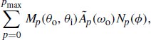
where Ãp are the normalized PDF terms. Note that θo must be shifted to account for hair scales when evaluating the PDF; this is done in the same way (and with the same code fragment) as with BSDF evaluation.
其中 à p 是标准化 PDF 项。请注意,在评估 PDF 时,必须移动 θ o 以考虑头发鳞片;这是以与 BSDF 评估相同的方式(并使用相同的代码片段)完成的。
〈Compute PDF for sampled hair scattering direction wi〉 ≡ Float pdf = 0; for (int p = 0; p < pMax; ++p) { 〈Compute sin θo and cos θo terms accounting for scales 617〉 〈Handle out-of-range cos θo from scale adjustment 617〉 pdf += Mp(cosTheta_i, cosThetap_o, sinTheta_i, sinThetap_o, v[p]) * apPDF[p] * Np(dphi, p, s, gamma_o, gamma_t); } pdf += Mp(cosTheta_i, cosTheta_o, sinTheta_i, sinTheta_o, v[pMax]) * apPDF[pMax] * (1 / (2 * Pi)); |
619 |
The HairBxDF::PDF() method performs the same computation and therefore the implementation is not included here.
HairBxDF::PDF() 方法执行相同的计算,因此这里不包括实现。
9.9.8 HAIR ABSORPTION COEFFICIENTS
9.9.8 毛发吸收系数
The color of hair is determined by how pigments in the cortex absorb light, which in turn is described by the normalized absorption coefficient where distance is measured in terms of the hair diameter. If a specific hair color is desired, there is a non-obvious relationship between the normalized absorption coefficient and the color of hair in a rendered image. Not only does changing the spectral values of the absorption coefficient have an unpredictable connection to the appearance of a single hair, but multiple scattering between collections of many hairs has a significant effect on each one’s apparent color. Therefore, pbrt provides implementations of two more intuitive ways to specify hair color.
头发的颜色是由皮层中的色素如何吸收光决定的,而这又是由归一化吸收系数描述的,其中距离是根据头发直径来测量的。如果需要特定的头发颜色,则归一化吸收系数和渲染图像中的头发颜色之间存在不明显的关系。改变吸收系数的光谱值不仅与单根毛发的外观具有不可预测的联系,而且许多毛发集合之间的多重散射对每根毛发的表观颜色也有显着影响。因此,pbrt 提供了两种更直观的方式来指定头发颜色的实现。
The first is based on the fact that the color of human hair is determined by the concentration of two pigments. The concentration of eumelanin is the primary factor that causes the difference between black, brown, and blonde hair. (Black hair has the most eumelanin and blonde hair has the least. White hair has none.) The second pigment, pheomelanin, causes hair to be orange or red. The HairBxDF class provides a convenience method that computes an absorption coefficient using the product of user-supplied pigment concentrations and absorption coefficients of the pigments.
第一个基于这样的事实:人类头发的颜色是由两种色素的浓度决定的。真黑色素的浓度是造成黑色、棕色和金色头发差异的主要因素。 (黑发含有最多的真黑素,金发含有最少。白发则没有。)第二种色素,褐黑素,使头发呈橙色或红色。 HairBxDF 类提供了一种方便的方法,该方法使用用户提供的颜料浓度和颜料吸收系数的乘积来计算吸收系数。
Float 23
浮法23
HairBxDF::Mp() 608
第608章
HairBxDF::Np() 615
第615章
HairBxDF::pMax 606
头发BxDF::pMax 606
HairBxDF::v 609
头发BxDF::v 609
Pi 1033
圆周率1033
Vector3f 86
矢量3f 86
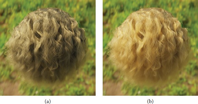
Figure 9.55: The Importance of Multiple Scattering in Blonde Hair. (a) Blonde hair rendered with up to three bounces of light inside the hair. (b) Rendered with up to fifty bounces of light. In light-colored hair, light that has been scattered many times makes an important contribution to its visual appearance. Accurately rendering very blonde or white hair is consequently more computationally intensive than rendering dark hair. (Hair geometry courtesy of Cem Yuksel.)
图 9.55:多重散射在金发中的重要性。 (a) 金色头发在头发内部最多反射三次光。 (b) 使用最多 50 次光反射进行渲染。在浅色头发中,多次散射的光对其视觉外观做出了重要贡献。因此,准确渲染非常金色或白色的头发比渲染深色头发的计算量更大。 (头发几何形状由 Cem Yuksel 提供。)
〈HairBxDF Method Definitions〉 +≡
〈HairBxDF 方法定义〉 +≡
RGBUnboundedSpectrum HairBxDF::SigmaAFromConcentration(Float ce, Float cp) {
RGB eumelaninSigma_a(0.419f, 0.697f, 1.37f);
RGB真黑色素Sigma_a(0.419f, 0.697f, 1.37f);
RGB pheomelaninSigma_a(0.187f, 0.4f, 1.05f);
RGB 褐黑素Sigma_a(0.187f, 0.4f, 1.05f);
RGB sigma_a = ce * eumelaninSigma_a + cp * pheomelaninSigma_a;
RGB sigma_a = ce * 真黑素Sigma_a + cp * 褐黑素Sigma_a;
return RGBUnboundedSpectrum(*RGBColorSpace::sRGB, sigma_a);
返回 RGBUnboundedSpectrum(*RGBColorSpace::sRGB, sigma_a);
}
Eumelanin concentrations of roughly 8, 1.3, and 0.3 give reasonable representations of black, brown, and blonde hair, respectively. Accurately rendering light-colored hair requires simulating many interreflections of light, however; see Figure 9.55.
真黑素浓度大约为 8、1.3 和 0.3,分别合理地代表了黑色、棕色和金色头发。然而,准确渲染浅色头发需要模拟许多光的相互反射;参见图 9.55。
It is also sometimes useful to specify the desired hair color directly; the SigmaAFromReflect ance() method, not included here, is based on a precomputed fit of absorption coefficients to scattered hair color.
有时直接指定所需的头发颜色也很有用; SigmaAFromReflect ance() 方法(此处未包含)基于吸收系数与散射头发颜色的预先计算拟合。
Hall’s (1989) book collected and described the state of the art in physically based surface reflection models for graphics; it remains a seminal reference. It discusses the physics of surface reflection in detail, with many pointers to the original literature.
Hall(1989)的书收集并描述了基于物理的图形表面反射模型的最新技术;它仍然是一个开创性的参考。它详细讨论了表面反射的物理原理,并引用了许多原始文献。
Microfacet Models
微面模型
Phong (1975) developed an early empirical reflection model for glossy surfaces in computer graphics. Although neither reciprocal nor energy conserving, it was a cornerstone of the first synthetic images of non-Lambertian objects. The Torrance–Sparrow microfacet model was described by Torrance and Sparrow (1967); it was first introduced to graphics by Blinn (1977), and a variant of it was used by Cook and Torrance (1981, 1982).
Phong (1975) 开发了计算机图形学中光泽表面的早期经验反射模型。虽然既不是倒数也不是能量守恒,但它是第一批非朗伯物体合成图像的基石。 Torrance-Sparrow 微面模型由 Torrance 和 Sparrow (1967) 描述; Blinn (1977) 首次将它引入图形学,Cook 和 Torrance (1981, 1982) 使用了它的一个变体。
Float 23
浮法23
RGB 182
RGBColorSpace::sRGB 186
RGB 颜色空间::sRGB 186
RGBUnboundedSpectrum 198
RGB无界光谱 198
The papers by Beckmann and Spizzichino (1963) and Trowbridge and Reitz (1975) introduced two widely used microfacet distribution functions. Kurt et al. (2010) introduced an anisotropic variant of the Beckmann–Spizzichino distribution function; see Heitz (2014) for anisotropic variants of many other microfacet distribution functions. (Early anisotropic BRDF models for computer graphics were developed by Kajiya (1985) and Poulin and Fournier (1990).) Ribardière et al. (2017) applied Student’s t-distribution to model microfacet distributions; it provides an additional degree of freedom, which they showed allows a better fit to measured data while subsuming both the Beckmann–Spizzichino and Trowbridge–Reitz distributions. Ribardière et al. (2019) investigated the connection between normal distribution functions (NDFs) and microfacet distributions and also showed how to generate surfaces with distributions described by their model.
Beckmann 和 Spizzichino (1963) 以及 Trowbridge 和 Reitz (1975) 的论文介绍了两种广泛使用的微面分布函数。库尔特等人。 (2010) 引入了 Beckmann-Spizzichino 分布函数的各向异性变体;有关许多其他微面分布函数的各向异性变体,请参阅 Heitz (2014)。 (计算机图形学的早期各向异性 BRDF 模型由 Kajiya (1985) 以及 Poulin 和 Fournier (1990) 开发。)Ribardière 等人。 (2017) 应用学生 t 分布来建模微面分布;它提供了额外的自由度,他们证明这可以更好地拟合测量数据,同时包含 Beckmann-Spizzichino 和 Trowbridge-Reitz 分布。里巴迪埃等人。 (2019) 研究了正态分布函数 (NDF) 和微面分布之间的联系,并展示了如何生成具有模型描述的分布的表面。
The microfacet masking-shadowing function was introduced by Smith (1967), building on the assumption that heights of nearby points on the microfacet surface are uncorrelated. Smith also first derived the normalization constraint in Equation (9.17). Heitz’s paper on microfacet masking-shadowing functions (2014) provides a very well-written introduction to microfacet BSDF models in general, with many useful figures and explanations about details of the topic.
微面掩蔽-阴影函数由 Smith (1967) 引入,其假设是微面表面上附近点的高度不相关。 Smith 还首先导出了方程(9.17)中的归一化约束。 Heitz 关于微面掩蔽-阴影函数的论文(2014 年)对微面 BSDF 模型进行了非常详尽的介绍,其中包含许多有用的图表和有关该主题细节的解释。
The more accurate G(ωi, ωo) function for Gaussian microfacet surfaces that better accounts for the effects of correlation between the two directions that we have implemented is due to Ross et al. (2005). Our derivation of the ∧(ω) function, Equation (9.19), follows Heitz (2015).
Ross 等人提出的高斯微面表面更准确的 G(ω, ω o ) 函数可以更好地解释我们所实现的两个方向之间相关性的影响。 (2005)。我们对 ∧(ω) 函数方程 (9.19) 的推导遵循 Heitz (2015)。
For many decades, Monte Carlo rendering of microfacet models involved generating samples proportional to the microfacet distribution D(ωh). Heitz and d’Eon (2014) were the first to demonstrate that it was possible to reduce variance by restricting this sampling process to only consider visible microfacets. Our microfacet sampling implementation in Section 9.6 follows Heitz’s improved approach (2018), which showed that sampling the visible area of the Trowbridge–Reitz microfacet distribution corresponds to sampling the projection of a truncated ellipsoid, which in turn can be performed using an approach developed by Walter et al. (2015). See also Heitz (2014) for an overview of traditional techniques that directly sample the microfacet distribution D(ωh) without considering visibility.
几十年来,微面模型的蒙特卡罗渲染涉及生成与微面分布 D(ω h ) 成比例的样本。 Heitz 和 d’Eon (2014) 第一个证明可以通过限制采样过程仅考虑可见的微面来减少方差。我们在第 9.6 节中的微面采样实现遵循 Heitz 的改进方法(2018),该方法表明对 Trowbridge-Reitz 微面分布的可见区域进行采样对应于对截断椭球体的投影进行采样,而这又可以使用由沃尔特等人。 (2015)。另请参阅 Heitz (2014),了解直接对微面分布 D(ω h ) 进行采样而不考虑可见性的传统技术的概述。
When dealing with refraction through rough dielectrics, a modified change of variables term is needed to account for the mapping from half vectors to outgoing direction. A model based on this approach was originally developed by Stam (2001); Walter et al. (2007) proposed improvements and provided an elegant geometric justification of the half vector mapping of Equation (9.36). The generalized half-direction vector for refraction used in these models and in Equation (9.34) is due to Sommerfeld and Runge (1911).
当处理通过粗糙电介质的折射时,需要修改变量项的变化来考虑从半矢量到出射方向的映射。基于这种方法的模型最初由 Stam (2001) 开发;沃尔特等人。 (2007) 提出了改进,并为方程 (9.36) 的半向量映射提供了优雅的几何论证。这些模型和方程 (9.34) 中使用的广义折射半方向矢量由 Sommerfeld 和 Runge (1911) 提出。
One issue with the specular term of the Torrance–Sparrow BRDF presented in Section 9.6.5 is that it only models a single scattering interaction with the microfacet surface, causing a growing portion of the energy to be lost as the roughness increases. In scenes where many subsequent interactions are crucial (e.g., a complex 3D object made from a translucent rough dielectric material), this energy loss can become so conspicuous that standard microfacet models become effectively unusable.
第 9.6.5 节中介绍的 Torrance-Sparrow BRDF 的镜面反射项的一个问题是,它仅模拟与微面表面的单次散射相互作用,导致随着粗糙度的增加,越来越多的能量损失。在许多后续交互至关重要的场景中(例如,由半透明粗糙介电材料制成的复杂 3D 对象),这种能量损失可能变得非常明显,以至于标准微面模型变得实际上无法使用。
The original model by Torrance and Sparrow (1967) included a diffuse component to simulate light having scattered multiple times. However, a simple diffuse correction is generally unsatisfactory, since the precise amount of energy loss will depend both on the surface roughness and the angle of incidence. Kelemen and Szirmay-Kalos (2001) proposed an improved diffuse-like term that accounts for this dependence. Jakob et al. (2014a) generalized their approach to rough dielectric boundaries in the context of layered structures, where energy losses can be particularly undesirable.
Torrance 和 Sparrow (1967) 的原始模型包含一个漫反射组件来模拟多次散射的光。然而,简单的漫射校正通常不能令人满意,因为能量损失的精确量将取决于表面粗糙度和入射角。 Kelemen 和 Szirmay-Kalos (2001) 提出了一个改进的类扩散项来解释这种依赖性。雅各布等人。 (2014a) 概括了他们在层状结构背景下处理粗糙介电边界的方法,其中能量损失可能特别不受欢迎。
In all of these cases, light is treated as essentially diffuse following scattering by multiple facets. Building on Smith’s uncorrelated height assumption, Heitz et al. (2016b) cast a microfacet BRDF model into a volumetric analogue composed of microflakes—that is, a distribution of mirror facets suspended in a 3D space. With this new interpretation, they are able to simulate an arbitrary number of volumetric scattering interactions to evaluate an effective BRDF that is free of energy loss and arguably closer to physical reality.
在所有这些情况下,光被多个面散射后基本上被视为漫射。基于史密斯的不相关高度假设,Heitz 等人。 (2016b) 将微面 BRDF 模型转换为由微薄片组成的体积模拟,即悬浮在 3D 空间中的镜面分布。通过这种新的解释,他们能够模拟任意数量的体积散射相互作用,以评估有效的 BRDF,该 BRDF 没有能量损失,并且可以说更接近物理现实。
Analytic solutions may sometimes obviate the need for a stochastic simulation of interreflection. For example, Lee et al. (2018) and Xie and Hanrahan (2018) both derived analytic models for multiple scattering under the assumption of microfacets with a v-groove shape. Efficient approximate models for multiple scattering among microfacets were presented by Kulla and Conty Estevez (2017) and by Turquin (2019).
解析解有时可能不需要相互反射的随机模拟。例如,李等人。 (2018) 以及 Xie 和 Hanrahan (2018) 都在假设微面具有 V 形槽形状的情况下导出了多重散射的分析模型。 Kulla 和 Conty Estevez (2017) 以及 Turquin (2019) 提出了微面之间多重散射的高效近似模型。
Microfacet models have provided a foundation for a variety of additional reflection models. Simonot (2009) has developed a model that spans Oren–Nayar’s diffuse microfacet model (1994) and Torrance–Sparrow: microfacets are modeled as Lambertian reflectors with a layer above them that ranges from perfectly transmissive to a perfect specular reflector. Conty Estevez and Kulla (2017) have developed a model for cloth. The halo of a softer and wider secondary highlight is often visible with rough surfaces. Barla et al. (2018) described a model for such surfaces with a focus on perceptually meaningful parameters for it.
Microfacet 模型为各种附加反射模型提供了基础。 Simonot (2009) 开发了一个涵盖 Oren–Nayar 的漫反射微面模型 (1994) 和 Torrance–Sparrow 的模型:微面被建模为朗伯反射器,其上方的层范围从完美透射到完美镜面反射器。 Conty Estevez 和 Kulla (2017) 开发了布料模型。在粗糙的表面上通常可以看到更柔和、更宽的次要高光的光晕。巴拉等人。 (2018)描述了此类表面的模型,重点关注其感知上有意义的参数。
Weyrich et al. (2009) have developed methods to infer a microfacet distribution that matches a measured or desired reflection distribution. Remarkably, they showed that it is possible to manufacture actual physical surfaces that match a desired reflection distribution fairly accurately.
魏里希等人。 (2009) 开发了推断与测量的或期望的反射分布相匹配的微面分布的方法。值得注意的是,他们表明可以制造相当准确地匹配所需反射分布的实际物理表面。
Layered Materials
分层材料
Many materials are naturally composed of multiple layers—for example, a metal base surface tarnished with patina, or wood with a varnish coating. Using a specialized BRDF to represent such structures can be vastly more efficient than resolving internal reflections using standard light transport methods.
许多材料天然地由多层组成,例如,失去光泽的金属基底表面或带有清漆涂层的木材。使用专门的 BRDF 来表示此类结构比使用标准光传输方法解决内反射要高效得多。
Hanrahan and Krueger (1993) modeled the layers of skin, accounting for just a single scattering event in each layer, and Dorsey and Hanrahan (1996) rendered layered materials using the Kubelka–Munk theory, which accounts for multiple scattering within layers but assumes that radiance distribution does not vary as a function of direction.
Hanrahan 和 Krueger (1993) 对皮肤层进行了建模,仅考虑了每层中的单个散射事件,而 Dorsey 和 Hanrahan (1996) 使用 Kubelka-Munk 理论渲染了分层材料,该理论考虑了层内的多次散射,但假设辐射分布不随方向而变化。
Pharr and Hanrahan (2000) showed that Monte Carlo integration could be used to solve the adding equations to efficiently compute BSDFs for layered materials without needing either of these simplifications. The adding equations are integral equations that accurately describe the effect of multiple scattering in layered media; they were derived by van de Hulst (1980) and Twomey et al. (1966).
Pharr 和 Hanrahan (2000) 表明,蒙特卡罗积分可用于求解加法方程,以有效计算层状材料的 BSDF,而无需进行这些简化。加法方程是积分方程,可以准确地描述层状介质中多重散射的影响;它们是由 van de Hulst (1980) 和 Twomey 等人推导出来的。 (1966)。
Weidlich and Wilkie (2007) rendered layered materials more efficiently by making a number of simplifying assumptions. Guo et al. (2018) showed that both unidirectional and bidirectional Monte Carlo random walks through layers led to efficient algorithms for evaluation, sampling, and PDF evaluation. (Their unidirectional approach is implemented in pbrt’s LayeredBxDF in Section 14.3.) Xia et al. (2020a) described an improved importance sampling for this approach and Gamboa et al. (2020) showed that bidirectional sampling was unnecessary and described a more efficient approach for multiple layers.
Weidlich 和 Wilkie (2007) 通过做出一些简化的假设,更有效地渲染了分层材料。郭等人。 (2018) 表明,单向和双向蒙特卡罗随机游走各层都会产生用于评估、采样和 PDF 评估的有效算法。 (他们的单向方法在第 14.3 节中的 pbrt 的 LayeredBxDF 中实现。)Xia 等人。 (2020a) 描述了该方法的改进重要性采样,Gamboa 等人。 (2020)表明双向采样是不必要的,并描述了一种更有效的多层方法。
LayeredBxDF 895
分层BxDF 895
Another approach for layered materials is to represent the aggregate scattering behavior of a layered surface using a parametric representation. Examples include Jakob et al. (2014a) and Zeltner and Jakob (2018), who applied the adding equations to discretized scattering matrices describing volumetric layers and rough interfaces. Guo et al. (2017) modeled coated surfaces using a modified microfacet scattering model. Belcour (2018) characterized individual layers’ scattering statistically, computed aggregate scattering using the adding equations, and then mapped the result to sums of lobes based on the Trowbridge–Reitz microfacet distribution function. Weier and Belcour (2020) generalized this approach to handle anisotropic reflection from the layer interfaces and Randrianandrasana et al. (2021) further generalized the model to improve accuracy and ensure energy conservation.
层状材料的另一种方法是使用参数表示来表示层状表面的聚集散射行为。例子包括雅各布等人。 (2014a) 以及 Zeltner 和 Jakob (2018),他们将加法方程应用于描述体积层和粗糙界面的离散散射矩阵。郭等人。 (2017) 使用改进的微面散射模型对涂层表面进行建模。 Belcour (2018) 对各个层的散射进行了统计表征,使用相加方程计算聚合散射,然后根据 Trowbridge-Reitz 微面分布函数将结果映射到波瓣总和。 Weier 和 Belcour(2020)推广了这种方法来处理来自层界面的各向异性反射,Randrianandrasana 等人。 (2021)进一步推广了该模型,以提高精度并确保节能。
It is possible to apply similar approaches to aggregate scattering at other scales. For example, Blumer et al. precomputed the effect of multiple scattering in complex geometry like trees and stored the result in a form that allows for efficient evaluation and sampling (Blumer et al. 2016).
可以将类似的方法应用于其他尺度的聚集散射。例如,布鲁默等人。预先计算了树等复杂几何体中多重散射的影响,并将结果存储为允许有效评估和采样的形式(Blumer 等人,2016)。
BSDF (Re-)Parameterization and Acquisition
BSDF(重新)参数化和采集
Improvements in data-acquisition technology have led to increasing amounts of detailed real-world BRDF data, even including BRDFs that are spatially varying (sometimes called “bidirectional texture functions,” BTFs) (Dana et al. 1999). See Müller et al. (2005) for a survey of work in BRDF measurement until the year 2005 and Guarnera et al. (2016) for a survey through the following decade.
数据采集技术的进步导致真实世界的 BRDF 数据的数量不断增加,甚至包括空间变化的 BRDF(有时称为“双向纹理函数”,BTF)(Dana 等人,1999)。参见穆勒等人。 (2005) 对 2005 年之前 BRDF 测量工作的调查,Guarnera 等人。 (2016)对接下来十年的调查。
Fitting measured BRDF data to parametric reflection models is a difficult problem. Rusinkiewicz (1998) made the influential observation that reparameterizing the measured data can make it substantially easier to compress or fit to models. The topic of BRDF parameterizations has also been investigated by Stark et al. (2005) and in Marscher’s Ph.D. dissertation (1998).
将测量的 BRDF 数据拟合到参数反射模型是一个难题。 Rusinkiewicz (1998) 做出了有影响力的观察,即重新参数化测量数据可以使压缩或拟合模型变得更加容易。 Stark 等人也研究了 BRDF 参数化的主题。 (2005) 和 Marscher 的博士学位。论文(1998)。
Building on Rusinkiewicz’s parameterization, Matusik et al. (2003a, 2003b) designed a BRDF representation and an efficient measurement device that repeatedly photographs a spherical sample to simultaneously acquire BRDF evaluations for many directions. They used this device to assemble a collection of isotropic material measurements that is now known as the MERL BRDF database. Baek et al. (2020) extended this approach with additional optics to capture polarimetric BRDFs, whose evaluation yields 4 × 4 Mueller matrices that characterize how reflection changes the polarization state of light. Nielsen et al. (2015) analyzed the manifold of MERL BRDFs to show that as few as 10–20 carefully chosen measurements can produce high-quality BRDF approximations.
Matusik 等人以 Rusinkiewicz 的参数化为基础。 ( 2003a, 2003b) 设计了一种 BRDF 表示方法和一种高效的测量装置,可以重复拍摄球形样本以同时获取多个方向的 BRDF 评估。他们使用该设备组装了各向同性材料测量的集合,现在称为 MERL BRDF 数据库。贝克等人。 (2020) 通过额外的光学器件扩展了这种方法,以捕获偏振 BRDF,其评估产生 4 × 4 Mueller 矩阵,用于表征反射如何改变光的偏振状态。尼尔森等人。 (2015) 分析了 MERL BRDF 的流形,表明只需 10-20 个精心选择的测量就可以产生高质量的 BRDF 近似值。
Dupuy et al. (2015) developed a simple iterative procedure for fitting standard microfacet distributions to measured BRDFs. Dupuy and Jakob (2018) generalized this procedure to arbitrary data-driven microfacet distributions and used the resulting approximation to perform a measurement in reparameterized coordinates, which is the approach underlying the MeasuredBxDF. They then used a motorized goniophotometer to spectroscopically acquire a collection of isotropic and anisotropic material samples that can be loaded into pbrt.
杜普伊等人。 (2015) 开发了一种简单的迭代程序,用于将标准微面分布拟合到测量的 BRDF。 Dupuy 和 Jakob(2018)将此过程推广到任意数据驱动的微面分布,并使用所得的近似值在重新参数化坐标中执行测量,这是 MeasuredBxDF 的基础方法。然后,他们使用电动测角光度计以光谱方式获取一系列各向同性和各向异性材料样本,并将其加载到 pbrt 中。
While the high-dimensional nature of reflectance functions can pose a serious impediment in any acquisition procedure, the resulting data can often be approximated much more compactly. Bagher et al. (2016) decomposed the MERL database into a set of 1D factors requiring 3.2 KiB per material. Vávra and Filip (2016) showed how lower-dimensional slices can inform a sparse measurement procedure for anisotropic materials.
虽然反射函数的高维性质可能对任何采集过程造成严重障碍,但所得数据通常可以更紧凑地近似。巴格尔等人。 (2016) 将 MERL 数据库分解为一组一维因子,每种材料需要 3.2 KiB。 Vávra 和 Filip (2016) 展示了低维切片如何为各向异性材料的稀疏测量程序提供信息。
MeasuredBxDF 592
测量dBxDF 592
Hair, Fur, and Fibers
头发、毛皮和纤维
Kajiya and Kay (1989) were the first to develop a reflectance model for hair fibers, observing the characteristic behavior of the underlying cylindrical reflectance geometry. For example, a thin and ideally specular cylinder under parallel illumination will reflect light into a 1D cone of angles. Reflection from a rough cylinder tends to concentrate around the specular 1D cone and decay with increasing angular distance. Kajiya and Kay proposed a phenomenological model combining diffuse and specular terms sharing these properties. For related work, see also the paper by Banks (1994), which discusses basic shading models for 1D primitives like hair. Goldman (1997) developed a probabilistic shading model that models reflection from collections of short hairs. Ward et al.’s survey (2007) has extensive coverage of early research in modeling, animating, and rendering hair.
Kajiya 和 Kay (1989) 第一个开发了头发纤维的反射率模型,观察了底层圆柱形反射率几何形状的特征行为。例如,平行照明下的薄且理想的镜面圆柱体会将光反射成一维锥角。来自粗糙圆柱体的反射往往集中在镜面一维锥体周围,并随着角距离的增加而衰减。 Kajiya 和 Kay 提出了一种现象学模型,结合了具有这些属性的漫反射和镜面反射项。有关相关工作,另请参阅 Banks (1994) 的论文,其中讨论了头发等一维图元的基本着色模型。 Goldman (1997) 开发了一种概率着色模型,用于模拟短毛集合的反射。 Ward 等人的调查(2007 年)广泛涵盖了头发建模、动画和渲染方面的早期研究。
Marschner et al. (2003) investigated the processes underlying scattering from hair and performed a variety of measurements of scattering from actual hair. They introduced the longitudinal/azimuthal decomposition and the use of the modified index of refraction to hair rendering. They then developed a scattering model where the longitudinal component was derived by first considering perfect specular paths and then allowing roughness by centering a Gaussian around them, and their azimuthal model assumed perfect specular reflections. They showed that this model agreed reasonably well with their measurements. Hery and Ramamoorthi (2012) showed how to sample the first term of this model and Pekelis et al. (2015) developed a more efficient approach to sampling all of its terms.
马施纳等人。 (2003) 研究了头发散射的过程,并对实际头发的散射进行了各种测量。他们引入了纵向/方位角分解以及使用修改后的折射率来渲染头发。然后,他们开发了一个散射模型,其中纵向分量是通过首先考虑完美的镜面反射路径,然后通过以它们为中心的高斯分布来允许粗糙度而导出的,并且他们的方位角模型假设完美的镜面反射。他们表明这个模型与他们的测量结果相当吻合。 Hery 和 Ramamoorthi (2012) 展示了如何对该模型的第一项进行采样,而 Pekelis 等人则展示了如何对该模型的第一项进行采样。 (2015)开发了一种更有效的方法来对其所有术语进行采样。
Zinke and Weber (2007) formalized different ways of modeling scattering from hair and clarified the assumptions underlying each of them. Starting with the bidirectional fiber scattering distribution function (BFSDF), which describes reflected differential radiance at a point on a hair as a fraction of incident differential power at another, they showed how assuming homogeneous scattering properties and a far-away viewer and illumination made it possible to simplify the eight-dimensional BFSDF to a four-dimensional bidirectional curve scattering distribution function (BCSDF). (Our implementation of the HairBxDF has glossed over some of these subtleties and opted for the simplicity of considering the scattering model as a BSDF.)
Zinke 和 Weber (2007) 形式化了头发散射建模的不同方法,并阐明了每种方法背后的假设。从双向光纤散射分布函数(BFSDF)开始,该函数将头发上一点的反射差分辐射率描述为另一点的入射差分功率的一部分,他们展示了假设均匀散射特性以及远处观察者和照明是如何实现这一点的可以将八维 BFSDF 简化为四维双向曲线散射分布函数(BCSDF)。 (我们对 HairBxDF 的实现掩盖了其中一些微妙之处,并选择简单地将散射模型视为 BSDF。)
Sadeghi et al. (2010) developed a hair scattering model with artist-friendly controls; Ou et al. (2012) showed how to sample from its distribution. Ogaki et al. (2010) created a tabularized model by explicitly modeling hair microgeometry and following random walks through it.
萨德吉等人。 (2010) 开发了一种具有艺术家友好控件的头发散射模型;欧等人。 (2012) 展示了如何从其分布中采样。大垣等人。 (2010) 通过显式建模头发微观几何形状并遵循随机游走创建了一个表格模型。
D’Eon et al. (2011, 2013) made a number of improvements to Marschner et al.’s model. They showed that their Mp term was not actually energy conserving and derived a new one that was; this is the model from Equation (9.49) that our implementation uses. (See also d’Eon (2013) for a more numerically stable formulation of Mp for low roughness, as well as Jakob (2012) for notes related to sampling their Mp term in a numerically stable way.) They also introduced a Gaussian to the azimuthal term, allowing for varying azimuthal roughness. A 1D quadrature method was used to integrate the model across the width of the hair h.
德翁等人。 (2011,2013)对Marschner等人的模型进行了一些改进。他们证明了他们的 M p 项实际上并不是能量守恒的,并推导出了一个新的项:这是我们的实现使用的方程 (9.49) 中的模型。 (另请参阅 d'Eon (2013),了解低粗糙度的 M p 数值更稳定的公式,以及 Jakob (2012),了解与采样 M p 项相关的注释以数值稳定的方式。)他们还在方位角项中引入了高斯函数,允许不同的方位角粗糙度。使用一维求积法对头发 h 宽度上的模型进行积分。
The RGB values used for the hair pigments in HairBxDF::SigmaAFromConcentration() were computed by d’Eon et al. (2011), based on a model by Donner and Jensen (2006). The function implemented in the HairBxDF::SigmaAFromReflectance() method is due to Chiang et al. (2016a), who created a cube of hair and rendered it with a variety of absorption coefficients and roughnesses while it was illuminated with a uniform white dome. They then fit a function that mapped from the hair’s azimuthal roughness and average color at the center of the front face of the cube to an absorption coefficient.
HairBxDF::SigmaAFromConcentration() 中用于头发色素的 RGB 值由 d’Eon 等人计算。 (2011),基于 Donner 和 Jensen (2006) 的模型。 HairBxDF::SigmaAFromReflectance() 方法中实现的函数归功于Chiang 等人。 (2016a),他创建了一个头发立方体,并用各种吸收系数和粗糙度对其进行渲染,同时用均匀的白色圆顶进行照明。然后,他们拟合一个函数,该函数将头发的方位粗糙度和立方体正面中心的平均颜色映射到吸收系数。
HairBxDF 606
头发BxDF 606
HairBxDF::SigmaAFromConcentration() 621
第621章
HairBxDF::SigmaAFromReflectance() 621
D’Eon et al. (2014) performed extensive Monte Carlo simulations of scattering from dielectric cylinders with explicitly modeled scales and glossy scattering at the boundary based on a Beckmann microfacet distribution. They showed that separable models did not model all the observed effects and that in particular the specular term modeled by Mp varies over the surface of the cylinder and also depends on ϕ. They developed a non-separable scattering model, where both α and βm vary as a function of h, and showed that it fit their simulations very accurately.
德翁等人。 (2014)基于贝克曼微面分布,对介电圆柱体的散射进行了广泛的蒙特卡罗模拟,具有明确建模的尺度和边界处的光泽散射。他们表明,可分离模型并没有对所有观察到的效果进行建模,特别是由 M p 建模的镜面反射项在圆柱体表面上变化,并且还取决于 phi。他们开发了一个不可分离的散射模型,其中 α 和 β m 都作为 h 的函数变化,并表明该模型非常准确地符合他们的模拟。
All the scattering models we have described so far have been BCSDFs—they represent the overall scattering across the entire width of the hair in a single model. Such “far field” models assume both that the viewer is far away and that incident illumination is uniform across the hair’s width. In practice, both of these assumptions are invalid if one is using path tracing to model multiple scattering inside hair. Two recent models have considered scattering at a single point along the hair’s width, making them more suitable for accurately modeling “near field” scattering.
到目前为止,我们描述的所有散射模型都是 BCSDF,它们代表单个模型中头发整个宽度上的整体散射。这种“远场”模型假设观察者距离很远,并且入射照明在整个头发的宽度上是均匀的。实际上,如果使用路径追踪来模拟头发内部的多重散射,这两种假设都是无效的。最近的两个模型考虑了沿头发宽度的单个点的散射,使它们更适合精确建模“近场”散射。
Yan et al. (2015) generalized d’Eon et al.’s model to account for scattering in the medulla, modeling a scattering cylinder in the interior of fur, and validated their model with a variety of measurements of actual animal fur. Subsequent work developed an efficient model that allows both near- and far-field evaluation (Yan et al. 2017a).
严等人。 (2015) 推广了 d’Eon 等人的模型来解释髓质中的散射,对毛皮内部的散射圆柱体进行建模,并通过对实际动物毛皮的各种测量来验证他们的模型。随后的工作开发了一种有效的模型,可以进行近场和远场评估(Yan et al. 2017a)。
Chiang et al. (2016a) showed that eliminating the integral over width from d’Eon et al.’s model works well in practice and that the sampling rates necessary for path tracing also worked well to integrate scattering over the curve width, giving a much more efficient implementation. They also developed the perceptually uniform parameterization of βm and βn that we have implemented in the HairBxDF as well as the inverse mapping from reflectance to σa used in our HairBxDF::SigmaAFromReflectance() method.
蒋等人。 (2016a) 表明,从 d'Eon 等人的模型中消除宽度积分在实践中效果很好,并且路径追踪所需的采样率也可以很好地积分曲线宽度上的散射,从而提供更有效的实现。他们还开发了我们在 HairBxDF 中实现的 β m 和 β n 的感知均匀参数化,以及使用的从反射率到 σ a 的逆映射在我们的 HairBxDF::SigmaAFromReflectance() 方法中。
Further recent advances in hair and fur rendering include work by Khungurn and Marschner (2017), who developed a scattering model from elliptical fibers and showed that modeling fibers as elliptical rather than cylindrical gives a closer match to measured data. Benamira and Pattanaik (2021) recently proposed a model that accounts for both elliptical fibers and diffraction effects, which are significant at the scale of human hair.
头发和毛皮渲染方面的最新进展包括 Kungurn 和 Marschner (2017) 的工作,他们开发了椭圆纤维的散射模型,并表明将纤维建模为椭圆形而不是圆柱形可以与测量数据更接近。 Benamira 和 Pattanaik (2021) 最近提出了一个模型,可以解释椭圆纤维和衍射效应,这在人类头发的尺度上非常重要。
Modeling and rendering the individual fibers of fabric is closely related to doing so for hair and fur. Recent work includes Zhao et al. (2016), who fit a procedural yarn model to CT-scanned yarn, and Aliaga et al. (2017), who demonstrated the complexity of scattering from a variety of cloth fibers and developed tabularized scattering functions for them using a precomputed simulation.
对织物的各个纤维进行建模和渲染与对头发和毛皮的建模和渲染密切相关。最近的工作包括赵等人。 (2016),他将程序纱线模型拟合到 CT 扫描纱线上,Aliaga 等人。 (2017),他展示了各种布料纤维散射的复杂性,并使用预先计算的模拟为其开发了表格化散射函数。
Glints and Microstructure
闪光和微观结构
The microfacet reflection models in this chapter are all based on the assumption that so many microfacets are visible in a pixel that they can be accurately described by their aggregate statistical behavior. This assumption is not true for many real-world surfaces, where a relatively small number of microfacets may be visible in each pixel; examples of such surfaces include glittery car paint and plastics. Additionally, many types of rough surfaces that aren’t considered glittery (e.g., bead-blasted plastic) are characterized by bright high-frequency glints under directionally peaked illumination (e.g., the sun).
本章中的微面反射模型均基于这样的假设:一个像素中可见如此多的微面,可以通过其聚合统计行为准确地描述它们。对于许多现实世界的表面来说,这种假设并不成立,其中每个像素中可能可见的微面数量相对较少;此类表面的例子包括闪闪发光的汽车油漆和塑料。此外,许多类型的粗糙表面不被认为是闪光的(例如,喷砂塑料),其特征是在定向峰值照明(例如,太阳)下会出现明亮的高频闪烁。
A common characteristic of many glint-rendering techniques is that they replace point evaluations of reflectance functions with a directional and/or spatial average covering a small region (e.g., a ray differential). With such an approach, a single sample suffices to find all glints visible within one pixel, which dramatically accelerates the rendering process.
许多闪烁渲染技术的一个共同特征是,它们用覆盖小区域的方向和/或空间平均值(例如光线微分)代替反射函数的点评估。通过这种方法,单个样本足以找到一个像素内所有可见的闪烁,这极大地加速了渲染过程。
HairBxDF 606
头发BxDF 606
HairBxDF::SigmaAFromReflectance() 621
One approach to rendering glints was introduced by Jakob et al. (2014b), who developed a temporally consistent stochastic process that samples glint positions on the fly during evaluation of a spatio-directional average. Wang et al. (2018) showed that the performance of this method could be improved by a separable approximation of the spatial and directional dimensions. These stochastic methods are compact but also very limited in terms of the glint distributions that can be modeled.
Jakob 等人提出了一种渲染闪烁的方法。 (2014b),他开发了一种时间一致的随机过程,可以在评估空间方向平均值时动态采样闪烁位置。王等人。 (2018)表明,可以通过空间和方向维度的可分离近似来提高该方法的性能。这些随机方法很紧凑,但在可建模的闪烁分布方面也非常有限。
In production rendering systems, fine surface details are often modeled using bump- or normal maps. Glinty surface appearance tends to result when such surfaces have high-resolution detail as well as a specular BRDF, and when they are furthermore subject to sharp (e.g., point or directional) illumination. At the same time, such configurations produce an extremely challenging Monte Carlo integration problem that has motivated numerous specialized methods for rendering normal-mapped specular surfaces.
在生产渲染系统中,精细的表面细节通常使用凹凸贴图或法线贴图进行建模。当此类表面具有高分辨率细节以及镜面 BRDF 时,并且当它们进一步受到锐利(例如,点或定向)照明时,往往会产生闪烁的表面外观。同时,这种配置产生了极具挑战性的蒙特卡罗积分问题,该问题激发了许多渲染法线贴图镜面表面的专门方法。
Yan et al. (2014) proposed a method that organizes the normal maps into a 4D spatiodirectional data structure that can be queried to find reflecting surface regions. Yan et al. (2016) drastically reduced the cost of reflectance queries by converting the normal map into a large superposition of 4D Gaussian functions termed a position-normal distribution. Though image fidelity is excellent, the overheads of these methods can be significant: slow rendering in the former case, and lengthy preprocessing and storage requirements in the second case. Zhu et al. (2019) addressed both of these issues via clustering and runtime synthesis of normal map detail. Wang et al. (2020a) substantially reduced the storage requirements by using a semi-procedural model that matches the statistics of an input texture. Zeltner et al. (2020) proposed a Newton-like equation-solving iteration that stochastically finds glints within texels of a normal map. Atanasov et al. (2021) developed a multi-level data structure for finding glints around a given half vector.
严等人。 (2014) 提出了一种将法线贴图组织成 4D 空间方向数据结构的方法,可以查询该数据结构以查找反射表面区域。严等人。 (2016) 通过将法线贴图转换为称为位置正态分布的 4D 高斯函数的大型叠加,大大降低了反射率查询的成本。尽管图像保真度非常好,但这些方法的开销可能很大:前一种情况下渲染速度较慢,后一种情况下需要冗长的预处理和存储要求。朱等人。 (2019) 通过法线贴图细节的聚类和运行时合成解决了这两个问题。王等人。 (2020a) 通过使用与输入纹理的统计数据相匹配的半过程模型,大大减少了存储需求。泽尔特纳等人。 (2020) 提出了一种类牛顿方程求解迭代,可以随机查找法线贴图纹理像素内的闪烁。阿塔纳索夫等人。 (2021)开发了一种多级数据结构,用于查找给定半向量周围的闪烁。
Other work in this area includes Raymond et al. (2016), who developed methods for rendering scratched surfaces, and Kuznetsov et al., who trained generative adversarial networks to represent microgeometry (Kuznetsov et al. 2019). Chermain et al. (2019) incorporated the effect of multiple scattering among the microstructure facets in such models, and Chermain et al. (2021) proposed a visible normal sampling technique for glint NDF. Loubet et al. recently developed a technique for sampling specular paths that is applicable to rendering caustics as well as rendering glints (2020).
该领域的其他工作包括 Raymond 等人。 (2016),开发了渲染划痕表面的方法;Kuznetsov 等人,训练生成对抗网络来表示微观几何形状 (Kuznetsov 等人,2019)。切尔曼等人。 (2019) 在此类模型中纳入了微观结构面之间的多重散射效应,Chermain 等人。 (2021) 提出了一种闪烁 NDF 的可见法线采样技术。卢贝特等人。最近开发了一种用于采样镜面反射路径的技术,该技术适用于渲染焦散以及渲染闪烁(2020)。
Wave Optics
波动光学
Essentially all physically based renderers are based on laws that approximate wave-optical behavior geometrically. At a high level, these approximations are sound given the large scale of depicted objects compared to the wavelength of light. At the same time, wave-optical properties tend to make themselves noticeable whenever geometric features occur at scales resembling the wavelength of light, and such features may indeed be present even on objects that are themselves drastically larger.
本质上,所有基于物理的渲染器都基于几何上近似波光学行为的定律。在较高的层面上,考虑到所描绘的物体与光的波长相比规模较大,这些近似值是合理的。与此同时,每当几何特征出现在类似于光波长的尺度上时,波动光学特性往往会变得引人注目,而且这些特征甚至可能确实存在于本身大得多的物体上。
For example, consider a thin film of oil on a puddle, a tiny scratch on an otherwise smooth metallic surface, or an object with micron-scale surface microstructure. These cases can feature striking structural coloration caused by the interference of light, which a purely geometric simulation would not be able to reproduce. It may be tempting to switch to a full wave-optical simulation of light in such cases, though this line of thought quickly runs into fundamental limits: for example, using the Finite Difference Time Domain (FDTD) method, the simulation domain would need to be discretized at resolutions of < 100 nm and simulated using sub-femtosecond timesteps. This can still work when studying local behavior at the micron scale, but it is practically infeasible for scenes measured in centimeters or even meters. These challenges have motivated numerous specialized methods that reintroduce such wave-optical effects within an otherwise geometric simulation.
例如,考虑水坑上的一层薄薄的油膜、光滑金属表面上的微小划痕或具有微米级表面微观结构的物体。这些案例可能具有由光干涉引起的引人注目的结构着色,这是纯粹的几何模拟无法再现的。在这种情况下,切换到光的全波光模拟可能很诱人,尽管这种思路很快就会遇到基本限制:例如,使用时域有限差分 (FDTD) 方法,模拟域需要以 < 100 nm 的分辨率进行离散化,并使用亚飞秒时间步长进行模拟。在研究微米尺度的局部行为时,这仍然有效,但对于以厘米甚至米为单位测量的场景实际上是不可行的。这些挑战激发了许多专门的方法,在其他几何模拟中重新引入这种波光效应。
Moravec (1981) was the first to apply a wave optics model to computer graphics. Other early work in this area includes Bahar and Chakrabarti (1987) and Stam (1999), who modeled diffraction effects from random and periodic structures. Cuypers et al. (2012) modeled multiple diffraction phenomena using signed BSDFs based on Wigner Distribution Functions.
Moravec (1981) 是第一个将波动光学模型应用于计算机图形学的人。该领域的其他早期工作包括 Bahar 和 Chakrabarti (1987) 以及 Stam (1999),他们对随机和周期性结构的衍射效应进行了建模。库珀斯等人。 (2012) 使用基于维格纳分布函数的带符号 BSDF 对多重衍射现象进行了建模。
Musbach et al. (2013) applied the FDTD to obtain a BRDF of the iridescent microstructure of a Morpho butterfly. Their paper provides extensive references to previous work on this topic. Dhillon et al. (2014) developed a model of diffraction from small-scale biological features such as are present in snake skin. Belcour and Barla (2017) modeled thin film iridescence on a rough microfacet surface and showed the importance of this effect for materials such as leather and how the resulting spectral variation can be efficiently calculated in an RGB-based simulation. Werner et al. (2017) developed a model for rendering surfaces with iridescent scratches. Yan et al. (2018) presented a surface microstructure model that integrates over a coherence area to produce iridescent glints, revealing substantial differences between geometric and wave-based modeling. Toisoul and Ghosh (2017) presented a method for capturing and reproducing the appearance of periodic grating-like structures. Xia et al. (2020b) showed that diffraction and interference are meaningful at the scale of fibers and developed a wave optics-based model for scattering from fibers that they validated with measured data.
穆斯巴赫等人。 (2013) 应用 FDTD 获得了 Morpho 蝴蝶虹彩微结构的 BRDF。他们的论文提供了对该主题先前工作的广泛参考。迪伦等人。 (2014)开发了一种小尺度生物特征(例如蛇皮中存在的特征)的衍射模型。 Belcour 和 Barla (2017) 对粗糙微表面上的薄膜虹彩进行了建模,并展示了这种效应对于皮革等材料的重要性,以及如何在基于 RGB 的模拟中有效计算由此产生的光谱变化。维尔纳等人。 (2017) 开发了一种用于渲染具有虹彩划痕的表面的模型。严等人。 (2018) 提出了一种表面微观结构模型,该模型在相干区域上集成以产生虹彩闪烁,揭示了几何建模和基于波的建模之间的实质性差异。 Toisoul 和 Ghosh (2017) 提出了一种捕获和再现周期性光栅状结构外观的方法。夏等人。 (2020b) 表明衍射和干涉在纤维尺度上是有意义的,并开发了一种基于波动光学的纤维散射模型,并用测量数据进行了验证。
In contrast to the above applications that reproduce dramatic goniochromatic effects, several works have studied how wave-based modeling can improve modeling of common materials (e.g., rough plastic or conductive surfaces). Löw et al. (2012) proposed and compared geometric and wave-based BRDF models in fits to materials to the MERL database. Dong et al. (2015) measured the surface microstructure of metal samples using a profilometer and used it to construct geometric and wave-based models that they then compared to goniophotometric measurements. Holzschuch and Pacanowski (2017) integrated diffraction effects into a microfacet model and showed that this gives a closer fit to measured data.
与上述再现戏剧性的角色效应的应用相比,一些工作研究了基于波的建模如何改进常见材料(例如粗糙的塑料或导电表面)的建模。勒夫等人。 (2012) 提出并比较了适合 MERL 数据库材料的几何和基于波的 BRDF 模型。董等人。 (2015) 使用轮廓仪测量金属样品的表面微观结构,并用它构建几何和基于波的模型,然后将其与测角光度测量进行比较。 Holzschuch 和 Pacanowski (2017) 将衍射效应集成到微面模型中,并表明这更接近测量数据。
Additional Topics
附加主题
The Lambertian BRDF is an idealized model; as noted earlier, it does not match many real-world BRDFs precisely. Oren and Nayar (1994) proposed an improved model based on Lambertian microfacets that allowed the specification of surface roughness. d’Eon has recently (2021) proposed a model based on scattering Lambertian spheres that matches the appearance of many materials well.
朗伯 BRDF 是一个理想化的模型;如前所述,它与现实世界中的许多 BRDF 并不完全匹配。 Oren 和 Nayar (1994) 提出了一种基于朗伯微面的改进模型,该模型允许指定表面粗糙度。 d’Eon 最近(2021)提出了一种基于散射朗伯球的模型,该模型与许多材料的外观很好地匹配。
A number of researchers have investigated BRDFs based on modeling the small-scale geometric features of a reflective surface. This work includes the computation of BRDFs from bump maps by Cabral, Max, and Springmeyer (1987); Fournier’s normal distribution functions (Fournier 1992); and a technique by Westin, Arvo, and Torrance (1992), who applied Monte Carlo ray tracing to statistically model reflection from microgeometry and represented the resulting BRDFs with spherical harmonics. Wu et al. (2011) developed a system that made it possible to model microgeometry and specify its underlying BRDF while interactively previewing the resulting macro-scale BRDF, and Falster et al. (2020) computed BSDFs of microgeometry, accounting for both multiple scattering and diffraction.
许多研究人员基于对反射表面的小尺度几何特征进行建模来研究 BRDF。这项工作包括 Cabral、Max 和 Springmeyer (1987) 根据凹凸贴图计算 BRDF; Fournier 的正态分布函数(Fournier 1992); Westin、Arvo 和 Torrance (1992) 提出的一项技术,他们应用蒙特卡罗射线追踪对微观几何反射进行统计建模,并用球谐函数表示所得的 BRDF。吴等人。 (2011) 开发了一个系统,可以对微观几何进行建模并指定其底层 BRDF,同时交互式预览生成的宏观尺度 BRDF,Falster 等人。 (2020) 计算了微观几何的 BSDF,同时考虑了多重散射和衍射。
The effect of the polarization of light is not modeled in pbrt, although for some scenes it can be an important effect; see, for example, the paper by Tannenbaum, Tannenbaum, and Wozny (1994) for information about how to extend a renderer to account for this effect. Fluorescence, where light is reflected at different wavelengths than the incident illumination, is also not modeled by pbrt; see Glassner (1994) and Wilkie et al. (2006) for more information on this topic.
光的偏振效应并未在 pbrt 中建模,尽管对于某些场景来说它可能是一个重要的效应;例如,请参阅 Tannenbaum、Tannenbaum 和 Wozny (1994) 的论文,了解有关如何扩展渲染器以解决此效果的信息。荧光(其中光以与入射照明不同的波长反射)也不是由 pbrt 建模的;参见 Glassner (1994) 和 Wilkie 等人。 (2006) 了解有关此主题的更多信息。
Modeling reflection from a variety of specific types of surfaces has received attention from researchers, leading to specialized reflection models. Examples include wood (Marschner, Westin, Arbree, and Moon 2005), car paint (Ergun et al. 2016), paper (Papas et al. 2014), and pearlescent materials (Guillén et al. 2020). Cloth remains a particularly challenging material to render; see the recent survey by Castillo et al. (2019) for comprehensive coverage of work in this area.
对各种特定类型表面的反射进行建模已受到研究人员的关注,从而产生了专门的反射模型。例子包括木材(Marschner、Westin、Arbree 和 Moon 2005)、汽车油漆(Ergun 等人,2016)、纸张(Papas 等人,2014)和珠光材料(Guillén 等人,2020)。布料仍然是一种渲染起来特别具有挑战性的材料;请参阅 Castillo 等人最近的调查。 (2019)全面报道该领域的工作。
Sampling BSDFs well is a key component of efficient image synthesis. Szécsi et al. (2003) evaluated different approaches for sampling BSDFs that are comprised of multiple lobes. It is often only possible to sample some factors of a BSDF (e.g., when sampling the Torrance–Sparrow BRDF using the distribution of visible microfacet normals); Herholz et al. fit parametric sampling distributions to BSDFs in an effort to sample them more effectively (Herholz et al. 2018).
良好的 BSDF 采样是高效图像合成的关键组成部分。塞奇等人。 (2003) 评估了对由多个波瓣组成的 BSDF 进行采样的不同方法。通常只能对 BSDF 的某些因子进行采样(例如,使用可见微面法线的分布对 Torrance-Sparrow BRDF 进行采样时);赫霍尔茨等人。将参数采样分布拟合到 BSDF,以更有效地对其进行采样(Herholz 等人,2018)。
pbrt’s test suite uses statistical hypothesis tests to verify the correctness of its BSDF sampling routines. The idea of verifying such graphics-related Monte Carlo sampling routines using statistical tests was introduced by Subr and Arvo (2007a). The χ2 test variant that is used in pbrt was originally developed as part of the Mitsuba renderer by Jakob (2010).
pbrt 的测试套件使用统计假设检验来验证其 BSDF 采样例程的正确性。 Subr 和 Arvo (2007a) 提出了使用统计测试验证此类与图形相关的蒙特卡洛采样例程的想法。 pbrt 中使用的 χ 2 测试变体最初由 Jakob (2010) 作为 Mitsuba 渲染器的一部分开发。
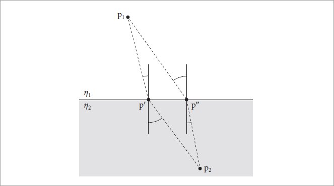
Figure 9.56: Derivation of Snell’s Law. Snell’s law can be derived using Fermat’s principle, which says that light will follow the path that takes the least amount of time to pass between two points. The angle of refraction θ at the boundary between two media can thus be shown to be the one that minimizes the time spent going from p1 to a point p on the boundary plus the time spent traveling the distance from that point to p2.
图 9.56:斯涅尔定律的推导。斯涅尔定律可以利用费马原理推导出来,该原理表示光将沿着在两点之间通过所需时间最短的路径移动。因此,两种介质之间边界处的折射角 θ 可以最小化从 p 1 到边界上的点 p 所花费的时间加上从该点行进的距离所花费的时间。指向 p 2 。
| ➊ 9.1 | A consequence of Fermat’s principle from optics is that light traveling from a point p1 in a medium with index of refraction η1 to a point p2 in a medium with index of refraction η2 will follow a path that minimizes the time to get from the first point to the second point. Snell’s law can be shown to follow directly from this fact. Consider light traveling between two points p1 and p2 separated by a planar boundary. The light could potentially pass through the boundary while traveling from p1 to p2 at any point on the boundary (see Figure 9.56, which shows two such possible points p′ and p″). Recall that the time it takes light to travel between two points in a medium with a constant index of refraction is proportional to the distance between them times the index of refraction in the medium. Using this fact, show that the point p′ on the boundary that minimizes the total time to travel from p1 to p2 is the point where η1 sin θ1 = η2 sin θ2. |
| ➋ 9.2 | Read the recent paper by d’Eon (2021) that describes a BRDF based on a model of the aggregate scattering of large collections of spherical particles that are themselves Lambertian. Implement this approach as a new BxDF in pbrt and render images comparing its visual appearance to that of the DiffuseBxDF. 阅读 d’Eon (2021) 最近发表的论文,该论文描述了基于大量球形粒子(本身就是朗伯粒子)的聚合散射模型的 BRDF。在 pbrt 中将此方法实现为新的 BxDF,并渲染图像,将其视觉外观与 DiffuseBxDF 的视觉外观进行比较。 |
| ➌ 9.3 | Read the paper of Wolff and Kurlander (1990) and the course notes of Wilkie and Weidlich (2012) and apply some of the techniques described to modify pbrt to model the effect of light polarization. (A more in-depth review of the principles of polarization is provided by Collett (1993).) Set up scenes and render images of them that demonstrate a significant difference when polarization is accurately modeled. For this, you will need to implement a polarized version of the Fresnel equations and add BSDFs that model optical elements like linear polarizers and retarders. 阅读 Wolff 和 Kurlander (1990) 的论文以及 Wilkie 和 Weidlich (2012) 的课程笔记,并应用所描述的一些技术来修改 pbrt 以模拟光偏振的效果。 (Collett (1993) 对偏振原理进行了更深入的回顾。)设置场景并渲染它们的图像,这些图像在精确建模偏振时表现出显着差异。为此,您需要实现菲涅尔方程的偏振版本,并添加对线性偏振器和延迟器等光学元件进行建模的 BSDF。 |
| ➌ 9.4 | Construct a scene with an actual geometric model of a rough plane with a large number of mirrored microfacets, and illuminate it with an area light source.11 Place the camera in the scene such that a very large number of microfacets are in each pixel’s area, and render images of this scene using hundreds or thousands of pixel samples. Compare the result to using a flat surface with a microfacet-based BRDF model. How well can you get the two approaches to match if you try to tune the microfacet BRDF parameters? Can you construct examples where images rendered with the true microfacets are actually visibly more realistic due to better modeling the effects of masking, self-shadowing, and interreflection between microfacets? 使用具有大量镜像微面的粗糙平面的实际几何模型构建场景,并使用区域光源对其进行照明。 11 将相机放置在场景中,使每个像素区域中有大量微面,并使用数百或数千个像素样本渲染该场景的图像。将结果与使用平面和基于微面的 BRDF 模型进行比较。如果您尝试调整微面 BRDF 参数,两种方法的匹配效果如何?您能否构造一些示例,其中由于更好地模拟了微面之间的遮蔽、自阴影和相互反射的效果,因此使用真实微面渲染的图像实际上明显更加真实? |
| ➌ 9.5 | One shortcoming of the microfacet-based BSDFs in this chapter is that they do not account for multiple scattering among microfacets. Investigate previous work in this area, including the stochastic multiple scattering model of Heitz et al. (2016b) and the analytic models of Lee et al. (2018) and Xie and Hanrahan (2018), and implement one of these approaches in pbrt. Then implement an approximate model for multiple scattering, such as the one presented by Kulla and Conty Estevez (2017) or by Turquin (2019). How do rendered images differ from pbrt’s current implementation? How closely do the approximate approaches match the more comprehensive ones? How does execution time compare? 本章中基于微面的 BSDF 的一个缺点是它们没有考虑微面之间的多重散射。研究该领域的先前工作,包括 Heitz 等人的随机多重散射模型。 (2016b) 和 Lee 等人的分析模型。 (2018) 和 Xie 和 Hanrahan (2018),并在 pbrt 中实现这些方法之一。然后实现多重散射的近似模型,例如 Kulla 和 Conty Estevez (2017) 或 Turquin (2019) 提出的模型。渲染图像与 pbrt 当前的实现有何不同?近似方法与更全面的方法的匹配程度如何?执行时间比较如何? |
| ➌ 9.6 | Review the algorithms for efficiently finding an approximation of a material’s normal distribution function and using that to measure BRDFs that are outlined in Section 9.8 and explained in more detail in Dupuy and Jakob (2018). Follow this approach to implement a virtual gonioreflectometer, where you provide pbrt with a description of the microgeometry of a complex surface (cloth, velvet, etc.) and its low-level reflection properties and then perform virtual measurements of the BSDF by simulating light paths in the microgeometry. Store the results of this simulation in the file format used by the MeasuredBxDFData and then render images that compare using the tabularized representation to directly rendering the microgeometry. How do the images compare? How much more computationally efficient is using the MeasuredBxDFData? BxDF 538 DiffuseBxDF 546 MeasuredBxDFData 598 |
| ➋ 9.7 | Marschner et al. (2003) note that human hair actually has an elliptical cross section that causes glints in human hair due to caustics; subsequent work by Khungurn and Marschner (2017) proposes a model that accounts for this effect and shows that it matches measurements of scattering from human hair well. Extend the HairBxDF implementation here, following their approach. One issue that you will need to address is that the ∂p/∂v returned by Curve::Intersect() is always perpendicular to the incident ray, which leads to different orientations of the azimuthal coordinate system. This is not an issue for the model we have implemented, since it operates only on the difference between angles ϕ in the hair coordinate system. For elliptical hairs, a consistent azimuthal coordinate system is necessary. 马施纳等人。 (2003) 请注意,人类的头发实际上具有椭圆形的横截面,这会导致人类的头发由于焦散而闪烁; Khungurn 和 Marschner (2017) 的后续工作提出了一个模型来解释这种效应,并表明它与人类头发散射的测量结果很好地匹配。按照他们的方法,在此处扩展 HairBxDF 实现。您需要解决的一个问题是 Curve::Intersect() 返回的 ∂p/∂v 始终垂直于入射光线,这导致方位角坐标系的方向不同。对于我们实现的模型来说,这不是问题,因为它仅对头发坐标系中角度 phi 之间的差进行操作。对于椭圆毛发,需要一致的方位角坐标系。 |
| ➌ 9.8 | Read Yan et al.’s paper on fur scattering (2015) and implement their model, which accounts for scattering in the medulla in fur. Render images that show the difference from accounting for this in comparison to the current implementation. You may want to also see Section 4.3 of Chiang et al. (2016a), which discusses extensions for modeling the undercoat (which is shorter and curlier hair underneath the top level) and a more ad hoc approach to account for the influence of scattering from the medulla. 阅读 Yan 等人关于毛皮散射的论文 (2015) 并实现他们的模型,该模型解释了毛皮髓质中的散射。渲染图像显示与当前实现相比考虑到这一点的差异。您可能还想查看Chiang 等人的第4.3 节。 (2016a),其中讨论了对底毛(顶层下方更短、更卷曲的毛发)进行建模的扩展,以及一种更特殊的方法来解释髓质散射的影响。 |
| ➌ 9.9 | Read one or more papers from the “Further Reading” section of this chapter on efficiently rendering glints, which are evident when the surface microstructure is large enough or viewed closely enough that the assumption of a continuous distribution of microfacet orientations is no longer valid. Then, choose one such approach and implement it in pbrt. Render images that show off the effects it is capable of producing. Curve::Intersect() 349 HairBxDF 606 |
_________________
1 It could be argued that a shortcoming of the BxDF sampling interface is that there are not entry points to sample from the 4D distribution of f(ω, ω′). This is a reasonably esoteric case for the applications envisioned for pbrt, however.
1 可以说,BxDF 采样接口的缺点是没有从 f(ω, ω′) 的 4D 分布中采样的入口点。然而,对于 pbrt 设想的应用程序来说,这是一个相当深奥的案例。
2 Strictly speaking, this is not always true: for example, the other method might also involve a delta distribution with matching direction ω′. pbrt does not consider this case, which may lead to a small loss of sampling efficiency in this rare corner case.
2 严格来说,这并不总是正确的:例如,另一种方法也可能涉及具有匹配方向 ω' 的 delta 分布。 pbrt 不考虑这种情况,这可能会导致在这种罕见的极端情况下采样效率略有损失。
3 See the online edition of the book for an additional chapter devoted to bidirectional light transport algorithms.
3 请参阅本书的在线版本,了解专门介绍双向光传输算法的附加章节。
4 The same model was also independently derived by Walter et al. (2007), who dubbed it “GGX.”
4 Walter 等人也独立推导了同一模型。 (2007),他将其称为“GGX”。
5 Both steps use ωi instead of ωi(k) to improve the smoothness of the interpolation.
5 两个步骤均使用 ω 代替 ω (k) 以提高插值的平滑度。
6 A repository of compatible files that cover the 360–1000 nm interval at roughly 4 nm resolution is available at http://rgl.epfl.ch/materials.
6 可在 http://rgl.epfl.ch/materials 上找到涵盖 360–1000 nm 间隔、分辨率约为 4 nm 的兼容文件存储库。
PiecewiseLinear2D 598
分段线性二维 598
7 Other authors generally include Ap in the Np term, though we find it more clear to keep them separate for the following exposition. Here we also use f for the BSDF, which most hair scattering papers denote by S.
7 其他作者通常将 A p 包含在 N p 项中,尽管我们发现在下面的说明中将它们分开会更清楚。这里我们也使用 f 来表示 BSDF,大多数毛发散射论文用 S 表示。
8 Note that this is a different usage of v than in earlier chapters when it was used for the parametric coordinate along the width of a curve.
8 请注意,这是 v 的用法与前面章节中的不同,当时它用于沿曲线宽度的参数坐标。
9 This is due to the Bravais properties of cylindrical scattering. See Appendix B of Marschner et al. (2003) for a derivation and further explanation.
9 这是由于柱面散射的布拉维特性。参见 Marschner 等人的附录 B。 (2003)的推导和进一步解释。
10 This approach is applicable since the BSDF’s definition includes the product of Mp and Np and so their joint PDF is separable.
10 这种方法是适用的,因为 BSDF 的定义包括 M p 和 N p 的乘积,因此它们的联合 PDF 是可分离的。
11 An area light and not a point or directional light is necessary due to subtleties in how lights are seen in specular surfaces. With the light transport algorithms used in pbrt, infinitesimal point sources are never visible in mirrored surfaces. This is a typical limitation of ray-tracing renderers and usually not bothersome in practice.
11 由于在镜面中观察光的方式存在微妙之处,因此需要使用区域光,而不是点光或定向光。通过 pbrt 中使用的光传输算法,无穷小的点源在镜面中永远不可见。这是光线追踪渲染器的典型限制,在实践中通常并不麻烦。