References
Adams, A., and M. Levoy. 2007. General linear cameras with finite aperture. In Rendering Techniques (Proceedings of the 2007 Eurographics Symposium on Rendering), 121–26.
Áfra, A. 2012. Incoherent ray tracing without acceleration structures. Eurographics 2012 Short Papers.
Áfra, A. T., C. Benthin, I. Wald, and J. Munkberg. 2016. Local shading coherence extraction for SIMD-efficient path tracing on CPUs. Proceedings of High Performance Graphics (HPG ’16), 119–28.
Ahmed, A., T. Niese, H. Huang, and O. Deussen. 2017. An adaptive point sampler on a regular lattice. ACM Transactions on Graphics (Proceedings of SIGGRAPH) 36 (4), 138:1–13.
Ahmed, A., H. Perrier, D. Coeurjolly, V. Ostromoukhov, J. Guo, D. Yan, H. Huang, and O. Deussen. 2016. Low-discrepancy blue noise sampling. ACM Transactions on Graphics (Proceedings of SIGGRAPH Asia) 35 (6), 247:1–13.
Ahmed, A. G. M., and P. Wonka. 2020. Screen-space blue-noise diffusion of Monte Carlo sampling error via hierarchical ordering of pixels. ACM Transactions on Graphics (Proceedings of SIGGRAPH Asia) 39 (6), 244:1–15.
Ahmed, A. G. M., and P. Wonka. 2021. Optimizing dyadic nets. ACM Transactions on Graphics (Proceedings of SIGGRAPH) 40 (4), 141:1–17.
Aila, T., and T. Karras. 2010. Architecture considerations for tracing incoherent rays. In Proceedings of High Performance Graphics 2010, 113–22.
Aila, T., T. Karras, and S. Laine. 2013. On quality metrics of bounding volume hierarchies. In Proceedings of High Performance Graphics 2013, 101–7.
Aila, T., and S. Laine. 2009. Understanding the efficiency of ray traversal on GPUs. In Proceedings of High Performance Graphics 2009, 145–50.
Akalin, F. 2015. Sampling the visible sphere. https://www.akalin.com/sampling-visible-sphere.
Akenine-Möller, T., C. Crassin, J. Boksansky, L. Belcour, A. Panteleev, and O. Wright. 2021. Improved shader and texture level of detail using ray cones. Journal of Computer Graphics Techniques (JCGT) 10 (1), 1–24.
Akenine-Möller, T., E. Haines, N. Hoffman, A. Peesce, M. Iwanicki, and S. Hillaire. 2018. Real-Time Rendering (4th ed.). Boca Raton, FL: CRC Press.
Akenine-Möller, T., J. Nilsson., M. Andersson, C. Barré-Brisebois, R. Toth, and T. Karras. 2019. Texture level of detail strategies for real-time ray tracing. In E. Haines and T. Akenine-Möller (ed.), Ray Tracing Gems, 321–45. Berkeley: Apress.
Aliaga, C., C. Castillo, D. Gutiérrez, M. A. Otaduy, J. Lopez-Moreno, and A. Jarabo. 2017. An appearance model for textile fibers. Computer Graphics Forum 36 (4), 35–45.
Alim, U. R. 2013. Rendering in shift-invariant spaces. In Proceedings of Graphics Interface 2013, 189–96.
Amanatides, J. 1984. Ray tracing with cones. Computer Graphics (SIGGRAPH ’84 Proceedings) 18 (3), 129–35.
Amanatides, J. 1992. Algorithms for the detection and elimination of specular aliasing. In Proceedings of Graphics Interface 1992, 86–93.
Amanatides, J., and D. P. Mitchell. 1990. Some regularization problems in ray tracing. In Proceedings of Graphics Interface 1990, 221–28.
Amanatides, J., and A. Woo. 1987. A fast voxel traversal algorithm for ray tracing. In Proceedings of Eurographics ’87, 3–10.
Ament, M., C. Bergmann, and D. Weiskopf. 2014. Refractive radiative transfer equation. ACM Transactions on Graphics (Proceedings of SIGGRAPH 2014) 33 (2), 17:1–22.
Anderson, L., T.-M. Li, J. Lehtinen, and F. Durand. 2017. Aether: An embedded domain specific sampling language for Monte Carlo rendering. ACM Transactions on Graphics (Proceedings of SIGGRAPH 2017) 36 (4), 99:1–16.
Anderson, S. 2004. Bit twiddling hacks. graphics.stanford.edu/~seander/bithacks.html.
Antonov, I. A., and V. M. Saleev. 1979. An economic method of computing LPτ sequences. Zh. Vychisl. Mat. Mat. Fiz. 19 (1), 243–45. (U.S.S.R. Computational Mathematics and Mathematical Physics 19 (1), 252–56.)
Apodaca, A. A., and L. Gritz. 2000. Advanced RenderMan: Creating CGI for Motion Pictures. San Francisco: Morgan Kaufmann.
Appel, A. 1968. Some techniques for shading machine renderings of solids. In AFIPS 1968 Spring Joint Computer Conference 32, 37–45.
Appleby, A. 2011. MurmurHash3. https://sites.google.com/site/murmurhash/.
Arnaldi, B., T. Priol, and K. Bouatouch. 1987. A new space subdivision method for ray tracing CSG modeled scenes. The Visual Computer 3 (2), 98–108.
Arvo, J. 1986. Backward ray tracing. In Developments in Ray Tracing, SIGGRAPH ’86 Course Notes, 259–63.
Arvo, J. 1988. Linear-time voxel walking for octrees. Ray Tracing News 1(5).
Arvo, J. 1990. Transforming axis-aligned bounding boxes. In A. S. Glassner (ed.), Graphics Gems I, 548–50. San Diego: Academic Press.
Arvo, J. 1993. Transfer equations in global illumination. In Global Illumination, SIGGRAPH ’93 Course Notes, Volume 42, 1:1–30.
Arvo, J. 1995a. Analytic methods for simulated light transport. Ph.D. thesis, Yale University.
Arvo, J. 1995b. Stratified sampling of spherical triangles. In Proceedings of SIGGRAPH 1995, 437–38.
Arvo, J. 2001a. Stratified sampling of 2-manifolds. In SIGGRAPH 2001 Course Notes 29, 1–34.
Arvo, J. 2001b. SphTri.h and SphTri.C. Jim Arvo’s Software and Data Archive, https://web.archive.org/web/20050216002912/http://www.cs.caltech.edu/~arvo/code/SphTri.C.
Arvo, J., and D. Kirk. 1987. Fast ray tracing by ray classification. Computer Graphics (SIGGRAPH ’87 Proceedings) 21(4), 55–64.
Arvo, J., and D. Kirk. 1990. Particle transport and image synthesis. Computer Graphics (SIGGRAPH ’90 Proceedings) 24 (4), 63–66.
Arvo, J., and K. Novins. 2007. Stratified sampling of convex quadrilaterals. Journal of Graphics, GPU, and Game Tools 12 (2), 1–12.
Ashdown, I. 1993. Near-field photometry: A new approach. Journal of the Illuminating Engineering Society 22 (1), 163–80.
Ashdown, I. 1994. Radiosity: A Programmer’s Perspective. New York: John Wiley & Sons.
Atanasov, A., V. Koylazov, B. Taskov, A. Soklev, V. Chizhov, and J. Křivánek. 2018. Adaptive environment sampling on CPU and GPU. In ACM SIGGRAPH 2018 Talks, 68:1–2.
Atanasov, A., A. Wilkie, V. Koylazov, and J. Křivánek. 2021. A multiscale microfacet model based on inverse bin mapping. Computer Graphics Forum (Proceedings of Eurographics) 40 (2), 103–13.
Atcheson, B., I. Ihrke, W. Heidrich, A. Tevs, D. Bradley, M. Magnor, and H.-P. Seidel. 2008. Time-resolved 3d capture of non-stationary gas flows. ACM Transactions on Graphics (Proceedings of SIGGRAPH Asia) 27 (5), 132:1–9.
Atkinson, K. 1993. Elementary Numerical Analysis. New York: John Wiley & Sons.
Azinović, D., T.-M. Li, A. Kaplanyan, and M. Nießner. 2019. Inverse path tracing for joint material and lighting estimation. In IEEE Conference on Computer Vision and Pattern Recognition, 2442–51.
Badouel, D., and T. Priol. 1990. An efficient parallel ray tracing scheme for highly parallel architectures. In Proceedings of the Fifth Eurographics conference on Advances in Computer Graphics Hardware: Rendering, Ray Tracing and Visualization Systems (EGGH ’90), 93–106.
Baek, S.-H., T. Zeltner, H. J. Ku, I. Hwang, X. Tong, W. Jakob, and M. H. Kim. 2020. Image-based acquisition and modeling of polarimetric reflectance. ACM Transactions on Graphics (Proceedings of SIGGRAPH) 39 (4), 139:1–14.
Bagher, M. M., J. M. Snyder, and D. Nowrouzezahrai. 2016. A non-parametric factor microfacet model for isotropic BRDFs. ACM Transactions on Graphics 35 (5), 159:1–16.
Bahar, E., and S. Chakrabarti. 1987. Full-wave theory applied to computer-aided graphics for 3D objects. IEEE Computer Graphics and Applications 7 (7), 46–60.
Bako, S., M. Meyer, T. DeRose, and P. Sen. 2019. Offline deep importance sampling for Monte Carlo path tracing. Computer Graphics Forum 38 (7), 527–42.
Bako, S., T. Vogels, B. McWilliams, M. Meyer, J. Novák, A. Harvill, P. Sen, T. DeRose, and F. Rousselle. 2017. Kernel-predicting convolutional networks for denoising Monte Carlo renderings. ACM Transactions on Graphics (Proceedings of SIGGRAPH) 36 (4), 97:1–14.
Bangaru, S., T.-M. Li, and F. Durand. 2020. Unbiased warped-area sampling for differentiable rendering. ACM Transactions on Graphics (Proceedings of SIGGRAPH Asia) 39 (6), 245:1–18.
Banks, D. C. 1994. Illumination in diverse codimensions. In Proceedings of SIGGRAPH ’94, Computer Graphics Proceedings, Annual Conference Series, 327–34.
Barequet, G., and G. Elber. 2005. Optimal bounding cones of vectors in three dimensions. Information Processing Letters 93 (2), 83–89.
Barkans, A. C. 1997. High-quality rendering using the Talisman architecture. In 1997 SIGGRAPH/Eurographics Workshop on Graphics Hardware, 79–88.
Barla, P., R. Pacanowski, and P. Vangorp. 2018. A composite BRDF model for hazy gloss. Computer Graphics Forum 37 (4), 55–66.
Barnes, C., and F.-L. Zhang. 2017. A survey of the state-of-the-art in patch-based synthesis. Computational Visual Media 3, 3–20.
Barnes, T. 2014. Exact bounding boxes for spheres/ellipsoids. https://tavianator.com/2014/ellipsoid_bounding_boxes.html.
Barringer, R., and T. Akenine-Möller. 2014. Dynamic ray stream traversal. ACM Transactions on Graphics (Proceedings of SIGGRAPH 2014) 33 (4), 151:1–9.
Barzel, R. 1997. Lighting controls for computer cinematography. Journal of Graphics Tools 2 (1), 1–20.
Bashford-Rogers, T., K. Debattista, and A. Chalmers. 2013. Importance driven environment map sampling. IEEE Transactions on Visualization and Computer Graphics 20 (6), 907–18.
Basu, K., and A. B. Owen. 2015. Low discrepancy constructions in the triangle. SIAM Journal on Numerical Analysis 53 (2), 743–61.
Basu, K., and A. B. Owen. 2016. Transformations and Hardy–Krause variation. SIAM Journal on Numerical Analysis 54 (3), 1946–66.
Basu, K., and A. B. Owen. 2017. Scrambled geometric net integration over general product spaces. Foundations of Computational Mathematics 17, 467–96.
Bauszat, P., M. Eisemann, and M. Magnor. 2010. The minimal bounding volume hierarchy. Vision, Modeling, and Visualization (2010), 227–34.
Becker, B. G., and N. L. Max. 1993. Smooth transitions between bump rendering algorithms. In Proceedings of SIGGRAPH ’93, Computer Graphics Proceedings, Annual Conference Series, 183–90.
Beckmann, P., and A. Spizzichino. 1963. The Scattering of Electromagnetic Waves from Rough Surfaces. New York: Pergamon.
Belcour, L. 2018. Efficient rendering of layered materials using an atomic decomposition with statistical operators. ACM Transactions on Graphics (Proceedings of SIGGRAPH) 37 (4), 73:1–15.
Belcour, L., and P. Barla. 2017. A practical extension to microfacet theory for the modeling of varying iridescence. ACM Transactions on Graphics (Proceedings of SIGGRAPH) 36 (4), 65:1–14.
Belcour, L., C. Soler, K. Subr, N. Holzschuch, and F. Durand. 2013. 5D covariance tracing for efficient defocus and motion blur. ACM Transactions on Graphics 32 (3), 31:1–18.
Belcour, L., G. Xie, C. Hery, M. Meyer, W. Jarosz, and D. Nowrouzezahrai. 2018. Integrating clipped spherical harmonics expansions. ACM Transactions on Graphics 37 (2), 19:1–12.
Belcour, L., L.-Q. Yan, R. Ramamoorthi, and D. Nowrouzezahrai. 2017. Antialiasing complex global illumination effects in path-space. ACM Transactions on Graphics 36 (1), 9:1–13.
Benamira, A., and S. Pattanaik. 2021. A combined scattering and diffraction model for elliptical hair rendering. Computer Graphics Forum (Proceedings of EGSR 2021) 40 (4), 163–75.
Benthin, C. 2006. Realtime ray tracing on current CPU architectures. Ph.D. thesis, Saarland University.
Benthin, C., S. Boulos, D. Lacewell, and I. Wald. 2007. Packet-based ray tracing of Catmull–Clark subdivision surfaces. SCI Institute Technical Report, No. UUSCI-2007-011. University of Utah.
Benthin, C., and I. Wald. 2009. Efficient ray traced soft shadows using multi-frusta tracing. In Proceedings of High Performance Graphics 2009, 135–44.
Benthin, C., I. Wald, and P. Slusallek. 2003. A scalable approach to interactive global illumination. In Computer Graphics Forum 22 (3), 621–30.
Benthin, C., I. Wald, and P. Slusallek. 2006. Techniques for interactive ray tracing of Bézier surfaces. Journal of Graphics, GPU, and Game Tools 11(2), 1–16.
Benthin, C., I. Wald, S. Woop, and A. T. Áfra. 2018. Compressed-leaf bounding volume hierarchies. Proceedings of High Performance Graphics (HPG ’18), 6:1–4.
Benthin, C., I. Wald, S. Woop, M. Ernst, and W. R. Mark. 2011. Combining single and packet ray tracing for arbitrary ray distributions on the Intel® MIC architecture. IEEE Transactions on Visualization and Computer Graphics 18 (9), 1438–48.
Benthin, C., S. Woop, M. Nießner, K. Selgrad, and I. Wald. 2015. Efficient ray tracing of subdivision surfaces using tessellation caching. Proceedings of the 7th Conference on High Performance Graphics (HPG ’15), 5–12.
Benthin, C., S. Woop, I. Wald, and A. T. Áfra. 2017. Improved two-level BVHs using partial re-braiding. Proceedings of High Performance Graphics (HPG ’17), 7:1–8.
Betrisey, C., J. F. Blinn, B. Dresevic, B. Hill, G. Hitchcock, B. Keely, D. P. Mitchell, J. C. Platt, and T. Whitted. 2000. Displaced filtering for patterned displays. Society for Information Display International Symposium. Digest of Technical Papers 31, 296–99.
Bhate, N., and A. Tokuta. 1992. Photorealistic volume rendering of media with directional scattering. In Proceedings of the Third Eurographics Rendering Workshop, 227–45.
Bigler, J., A. Stephens, and S. Parker. 2006. Design for parallel interactive ray tracing systems. IEEE Symposium on Interactive Ray Tracing, 187–95.
Bikker, J., and J. van Schijndel. 2013. The Brigade renderer: A path tracer for real-time games. International Journal of Computer Games Technology, Volume 8.
Billen, N., and P. Dutré. 2016. Line sampling for direct illumination. Computer Graphics Forum 35 (4), 45–55.
Billen, N., B. Engelen, A. Lagae, and P. Dutré. 2013. Probabilistic visibility evaluation for direct illumination. Computer Graphics Forum (Proceedings of the 2013 Eurographics Symposium on Rendering) 32 (4), 39–47.
Billen, N., A. Lagae, and P. Dutré. 2014. Probabilistic visibility evaluation using geometry proxies. Computer Graphics Forum (Proceedings of the 2014 Eurographics Symposium on Rendering) 33 (4), 143–52.
Binder, N., and A. Keller. 2016. Efficient stackless hierarchy traversal on GPUs with backtracking in constant time. Proceedings of High Performance Graphics, 41–50.
Binder, N., and A. Keller. 2018. Fast, high precision ray/fiber intersection using tight, disjoint bounding volumes. arXiv:1811.03374 [cs.GR].
Binder, N., and A. Keller. 2020. Massively parallel construction of radix tree forests for the efficient sampling of discrete or piecewise constant probability distributions. Monte Carlo and Quasi-Monte Carlo Methods (MCQMC 2018). arXiv: 1902.05942 [cs].
Bitterli, B., W. Jakob, J. Novák, and W. Jarosz. 2018a. Reversible jump Metropolis light transport using inverse mappings. ACM Transactions on Graphics 37 (1), 1:1–12.
Bitterli, B., and W. Jarosz. 2019. Selectively Metropolised Monte Carlo light transport simulation. ACM Transactions on Graphics (Proceedings of SIGGRAPH Asia) 38 (6), 153:1–10.
Bitterli, B., J. Novák, and W. Jarosz. 2015. Portal-masked environment map sampling. Computer Graphics Forum (Proceedings of the 2015 Eurographics Symposium on Rendering) 34 (4), 13–19.
Bitterli, B., S. Ravichandran, T. Müller, M. Wrenninge, J. Novák, S. Marschner, and W. Jarosz. 2018b. A radiative transfer framework for non-exponential media. ACM Transactions on Graphics (Proceedings of SIGGRAPH Asia) 37 (6), 225:1–17.
Bitterli, B., F. Rousselle, B. Moon, J. A. Iglesias-Guitián, D. Adler, K. Mitchell, W. Jarosz, and J. Novák. 2016. Nonlinearly weighted first-order regression for denoising Monte Carlo renderings. Computer Graphics Forum 35 (4), 107–17.
Bitterli, B., C. Wyman, M. Pharr, P. Shirley, A. Lefohn, and W. Jarosz. 2020. Spatiotemporal reservoir resampling for real-time ray tracing with dynamic direct lighting. ACM Transactions on Graphics (Proceedings of SIGGRAPH) 39 (4), 148:1–17.
Bittner, J., M. Hapala, and V. Havran. 2013. Fast insertion-based optimization of bounding volume hierarchies. Computer Graphics Forum 32 (1), 85–100.
Bittner, J., M. Hapala, and V. Havran. 2014. Incremental BVH construction for ray tracing. Computers & Graphics 47, 135–44.
Bjorke, K. 2001. Using Maya with RenderMan on Final Fantasy: The Spirits Within. SIGGRAPH 2001 RenderMan Course Notes.
Blakey, E. 2012. Ray tracing—computing the incomputable? Developments in Computational Models, 32–40.
Blasi, P., B. L. Saëc, and C. Schlick. 1993. A rendering algorithm for discrete volume density objects. Computer Graphics Forum (Proceedings of Eurographics ’93) 12 (3), 201–10.
Blinn, J. F. 1977. Models of light reflection for computer synthesized pictures. Computer Graphics (SIGGRAPH ’77 Proceedings) 11, 192–98.
Blinn, J. F. 1978. Simulation of wrinkled surfaces. In Computer Graphics (SIGGRAPH ’78 Proceedings) 12, 286–92.
Blinn, J. F. 1982a. A generalization of algebraic surface drawing. ACM Transactions on Graphics 1(3), 235–56.
Blinn, J. F. 1982b. Light reflection functions for simulation of clouds and dusty surfaces. Computer Graphics 16 (3), 21–29.
Blinn, J. F., and M. E. Newell. 1976. Texture and reflection in computer generated images. Communications of the ACM 19, 542–46.
Blumer, A., J. Novák, R. Habel, D. Nowrouzezahrai, and W. Jarosz. 2016. Reduced aggregate scattering operators for path tracing. Computer Graphics Forum 35 (7), 461–73.
Blumofe, R., C. Joerg, B. Kuszmaul, C. Leiserson, K. Randall, and Y. Zhou. 1996. Cilk: An efficient multithreaded runtime system. Journal of Parallel and Distributed Computing 37 (1), 55–69.
Blumofe, R., and C. Leiserson. 1999. Scheduling multithreaded computations by work stealing. Journal of the ACM 46 (5), 720–48.
Boehm, H.-J. 2005. Threads cannot be implemented as a library. ACM SIGPLAN Notices 40 (6), 261–68.
Boksansky, J., C. Crassin, and T. Akenine-Möller. 2021. Refraction ray cones for texture level of detail. In Marrs, A., P. Shirley, and I. Wald (eds.), Ray Tracing Gems II. Berkeley: Apress, 127–38.
Borges, C. 1991. Trichromatic approximation for computer graphics illumination models. Computer Graphics (Proceedings of SIGGRAPH ’91) 25, 101–4.
Bouchard, G., J.-C. Iehl, V. Ostromoukhov, and P. Poulin. 2013. Improving robustness of Monte-Carlo global illumination with directional regularization. In SIGGRAPH Asia 2013 Technical Briefs, 22:1–4.
Boughida, M., and T. Boubekeur. 2017. Bayesian collaborative denoising for Monte Carlo rendering. Computer Graphics Forum 36 (4), 137–53.
Boulos, S., and E. Haines. 2006. Ray–box sorting. Ray Tracing News 19 (1), www.realtimerendering.com/resources/RTNews/html/rtnv19n1.html.
Boulos, S., I. Wald, and C. Benthin. 2008. Adaptive ray packet reordering. In Proceedings of IEEE Symposium on Interactive Ray Tracing, 131–38.
Braaten, E., and G. Weller. 1979. An improved low-discrepancy sequence for multidimensional quasi-Monte Carlo integration. Journal of Computational Physics 33 (2), 249–58.
Bracewell, R. N. 2000. The Fourier Transform and Its Applications. New York: McGraw-Hill.
Bratley, P., and B. L. Fox. 1988. Algorithm 659: Implementing Sobol’s quasirandom sequence generator. ACM Transactions on Mathematical Software 14 (1), 88–100.
Bresenham, J. E. 1965. Algorithm for computer control of a digital plotter. IBM Systems Journal 4 (1), 25–30.
Bronsvoort, W. F., and F. Klok. 1985. Ray tracing generalized cylinders. ACM Transactions on Graphics 4 (4), 291–303.
Bruneton, E. 2017. A qualitative and quantitative evaluation of 8 clear sky models. IEEE Transactions on Visualization and Computer Graphics 23 (12), 2641–55.
Bruneton, E., and F. Neyret. 2012. A survey of nonlinear prefiltering methods for efficient and accurate surface shading. IEEE Transactions on Visualization and Computer Graphics 18 (2), 242–60.
Buck, R. C. 1978. Advanced Calculus. New York: McGraw-Hill.
Budge, B., T. Bernardin, J. Stuart, S. Sengupta, K. Joy, and J. D. Owens. 2009. Out-of-core data management for path tracing on hybrid resources. Computer Graphics Forum (Proceedings of Eurographics 2009) 28 (2), 385–96.
Budge, B., D. Coming, D. Norpchen, and K. Joy. 2008. Accelerated building and ray tracing of restricted BSP trees. 2008 IEEE Symposium on Interactive Ray Tracing, 167–74.
Buisine, J., S. Delepoulle, and C. Renaud. 2021. Firefly removal in Monte Carlo rendering with adaptive Median of meaNs. Proceedings of the Eurographics Symposium on Rendering, 121–32.
Burke, D., A. Ghosh, and W. Heidrich. 2005. Bidirectional importance sampling for direct illumination. In Rendering Techniques 2005: 16th Eurographics Workshop on Rendering, 147–56.
Burley, B. 2012. Physically-based shading at Disney. Physically Based Shading in Film and Game Production, SIGGRAPH 2012 Course Notes.
Burley, B. 2020. Hash-based Owen scrambling. Journal of Computer Graphics Techniques (JCGT) 9 (4), 1–20.
Burley, B., D. Adler, M. J-Y. Chiang, H. Driskill, R. Habel, P. Kelly, P. Kutz, Y. K. Li, and D. Teece. 2018. The design and evolution of Disney’s Hyperion renderer. ACM Transactions on Graphics 37 (3), 33:1–22.
Cabral, B., N. Max, and R. Springmeyer. 1987. Bidirectional reflection functions from surface bump maps. Computer Graphics (SIGGRAPH ’87 Proceedings) 21, 273–81.
Cant, R. J., and P. A. Shrubsole. 2000. Texture potential MIP mapping, a new high-quality texture antialiasing algorithm. ACM Transactions on Graphics 19 (3), 164–84.
Carr, N., J. D. Hall, and J. Hart. 2002. The ray engine. In Proceedings of ACM SIGGRAPH Workshop on Graphics Hardware 2002, 37–46.
Castillo, C., J. López-Moreno, and C. Aliaga. 2019. Recent advances in fabric appearance reproduction. Computers & Graphics 84, 103–21.
Catmull, E., and J. Clark. 1978. Recursively generated B-spline surfaces on arbitrary topological meshes. Computer-Aided Design 10, 350–55.
Cazals, F., G. Drettakis, and C. Puech. 1995. Filtering, clustering and hierarchy construction: A new solution for ray-tracing complex scenes. Computer Graphics Forum 14 (3), 371–82.
Celarek, A., W. Jakob, M. Wimmer, and J. Lehtinen. 2019. Quantifying the error of light transport algorithms. Computer Graphics Forum 38 (4), 111–21.
Cerezo, E., F. Perez-Cazorla, X. Pueyo, F. Seron, and F. Sillion. 2005. A survey on participating media rendering techniques. The Visual Computer 21(5), 303–28.
Chaitanya, C. R. A., A. S. Kaplanyan, C. Schied, M. Salvi, A. Lefohn, D. Nowrouzezahrai, and T. Aila. 2017. Interactive reconstruction of Monte Carlo image sequences using a recurrent denoising autoencoder. ACM Transactions on Graphics (Proceedings of SIGGRAPH) 36 (4), 98:1–12.
Chan, T. F., G. Golub, R. J. LeVeque. 1979. Updating formulae and a pairwise algorithm for computing sample variances. Technical Report STAN-CS-79-773, Department of Computer Science, Stanford University.
Chandrasekhar, S. 1960. Radiative Transfer. New York: Dover Publications. Originally published by Oxford University Press, 1950.
Chao, M. T. 1982. A general purpose unequal probability sampling plan. Biometrika 69 (3), 653–56.
Chen, J., K. Venkataraman, D. Bakin, B. Rodricks, R. Gravelle, P. Rao, and Y. Ni. 2009. Digital camera imaging system simulation. IEEE Transactions on Electron Devices 56 (11), 2496–505.
Chen, H. C., and Y. Asau. 1974. On generating random variates from an empirical distribution. AIIE Transactions 6 (2), 163–66.
Chen, Q., and V. Koltun. 2017. Photographic image synthesis with cascaded refinement networks. IEEE/CVF International Conference on Computer Vision (ICCV), 1511–20. arXiv:1707:09405 [cs.CV].
Chen, X., D. Cohen-Or, B. Chen, and N. J. Mitra. 2021. Towards a neural graphics pipeline for controllable image generation. Computer Graphics Forum 40 (2), 127–40.
Chermain, X., F. Claux, and S. Mérillou. 2019. Glint rendering based on a multiple-scattering patch BRDF. Computer Graphics Forum 38 (4), 27–37.
Chermain, X., B. Sauvage, J.-M. Dischler, and C. Dachsbacher. 2021. Importance sampling of glittering BSDFs based on finite mixture distributions. Proceedings of the Eurographics Symposium on Rendering, 45–53.
Chiang, M. J.-Y., B. Bitterli, C. Tappan, and B. Burley. 2016a. A practical and controllable hair and fur model for production path tracing. Computer Graphics Forum (Proceedings of Eurographics 2016) 35 (2), 275–83.
Chiang, M. J.-Y., P. Kutz, and B. Burley. 2016b. Practical and controllable subsurface scattering for production path tracing. ACM SIGGRAPH 2016 Talks, 49:1–2.
Chiang, M. J.-Y., Y. K. Li, and B. Burley. 2019. Taming the shadow terminator. ACM SIGGRAPH 2019 Talks, 71:1–2.
Chiu, K., P. Shirley, and C. Wang. 1994. Multi-jittered sampling. In P. Heckbert (ed.), Graphics Gems IV, 370–74. San Diego: Academic Press.
Cho, I.-Y., Y. Huo, and S.-E. Yoon. 2021. Weakly-supervised contrastive learning in path manifold for Monte Carlo image reconstruction. ACM Transactions on Graphics (Proceedings of SIGGRAPH 2021) 40 (4), 38:1–14.
Choi, B., B. Chang, and I. Ihm. 2013. Improving memory space efficiency of kd-tree for real-time ray tracing. Computer Graphics Forum 32 (7), 335–44.
Choi, B., R. Komuravelli, V. Lu, H. Sung, R. L. Bocchino, S. V. Adve, and J. C. Hart. 2010. Parallel SAH k-D tree construction. In Proceedings of High Performance Graphics 2010, 77–86.
Christensen, P. 2015. The path-tracing revolution in the movie industry. ACM SIGGRAPH 2015 Course, 24:1–7.
Christensen, P. 2018. Progressive sampling strategies for disk light sources. Pixar Animation Studios Technical Memo 18-02.
Christensen, P., J. Fong, J. Shade, W. Wooten, B. Schubert, A. Kensler, S. Friedman, C. Kilpatrick, C. Ramshaw, M. Bannister, B. Rayner, J. Brouillat, and M. Liani. 2018. RenderMan: An advanced path-tracing architecture for movie rendering. ACM Transactions on Graphics 37 (3), 30:1–21.
Christensen, P., A. Kensler, and C. Kilpatrick. 2018. Progressive multi-jittered sample sequences. Computer Graphics Forum 37 (4), 21–33.
Christensen, P. H. 2003. Adjoints and importance in rendering: An overview. IEEE Transactions on Visualization and Computer Graphics 9 (3), 329–40.
Christensen, P. H., J. Fong, D. M. Laur, and D. Batali. 2006. Ray tracing for the movie Cars. In Proceedings of the IEEE Symposium on Interactive Ray Tracing, 1–6.
Christensen, P. H., D. M. Laur, J. Fong, W. L. Wooten, and D. Batali. 2003. Ray differentials and multiresolution geometry caching for distribution ray tracing in complex scenes. In Computer Graphics Forum (Eurographics 2003 Conference Proceedings) 22 (3), 543–52.
CIE Technical Report. 2004. Colorimetry. Publication 15:2004 (3rd ed.), CIE Central Bureau, Vienna.
Ciechanowski, B. 2019. Color spaces. https://ciechanow.ski/color-spaces/.
Cigolle, Z. H., S. Donow, D. Evangelakos, M. Mara, M. McGuire, and Q. Meyer. 2014. Survey of efficient representations for independent unit vectors. Journal of Computer Graphics Techniques (JCGT) 3 (2), 1–30.
Clarberg, P. 2008. Fast equal-area mapping of the (hemi)sphere using SIMD. Journal of Graphics Tools 13 (3), 53–68.
Clarberg, P., and T. Akenine-Möller. 2008a. Practical product importance sampling for direct illumination. Computer Graphics Forum (Proceedings of Eurographics 2008) 27 (2), 681–90.
Clarberg, P., and T. Akenine-Möller. 2008b. Exploiting visibility correlation in direct illumination. Computer Graphics Forum (Proceedings of the 2008 Eurographics Symposium on Rendering) 27 (4), 1125–36.
Clarberg, P., W. Jarosz, T. Akenine-Möller, and H. W. Jensen. 2005. Wavelet importance sampling: Efficiently evaluating products of complex functions. ACM Transactions on Graphics (Proceedings of SIGGRAPH 2005) 24 (3), 1166–75.
Clark, J. H. 1976. Hierarchical geometric models for visible surface algorithms. Communications of the ACM 19 (10), 547–54.
Cleary, J. G., B. M. Wyvill, R. Vatti, and G. M. Birtwistle. 1983. Design and analysis of a parallel ray tracing computer. In Proceedings of Graphics Interface 1983, 33–38.
Cleary, J. G., and G. Wyvill. 1988. Analysis of an algorithm for fast ray tracing using uniform space subdivision. The Visual Computer 4 (2), 65–83.
Cline, D., D. Adams, and P. Egbert. 2008. Table-driven adaptive importance sampling. Computer Graphics Forum (Proceedings of the 2008 Eurographics Symposium on Rendering) 27 (4), 1115–23.
Cline, D., P. Egbert, J. Talbot, and D. Cardon. 2006. Two stage importance sampling for direct lighting. Rendering Techniques 2006: 17th Eurographics Workshop on Rendering, 103–14.
Cline, D., A. Razdan, and P. Wonka. 2009. A comparison of tabular PDF inversion methods. Computer Graphics Forum 28 (1), 154–60.
Clinton, A., and M. Elendt. 2009. Rendering volumes with microvoxels. SIGGRAPH 2009 Talks, 47:1.
Cohen, J., M. Olano, and D. Manocha. 1998. Appearance-preserving simplification. In Proceedings of SIGGRAPH ’98, Computer Graphics Proceedings, Annual Conference Series, 115–22.
Cohen, J., A. Varshney, D. Manocha, G. Turk, H. Weber, P. Agarwal, F. P. Brooks Jr., and W. Wright. 1996. Simplification envelopes. In Proceedings of SIGGRAPH ’96, Computer Graphics Proceedings, Annual Conference Series, 119–28.
Cohen, M., and D. P. Greenberg. 1985. The hemi-cube: A radiosity solution for complex environments. SIGGRAPH Computer Graphics 19 (3), 31–40.
Cohen, M., and J. Wallace. 1993. Radiosity and Realistic Image Synthesis. San Diego: Academic Press Professional.
Collett, E. 1993. Polarized Light: Fundamentals and Applications. New York: Marcel Dekker.
Collins, S. 1994. Adaptive splatting for specular to diffuse light transport. In Fifth Eurographics Workshop on Rendering, 119–35.
Conty Estevez, A., and C. Kulla. 2017. Production friendly microfacet sheen BRDF. SIGGRAPH 2017 Talks.
Conty Estevez, A., and C. Kulla. 2018. Importance sampling of many lights with adaptive tree splitting. Proceedings of the ACM on Computer Graphics and Interactive Techniques 1(2), 25:1–17.
Conty Estevez, A., and C. Kulla. 2020. Adaptive caustics rendering in production with photon guiding. EGSR Industry Track.
Conty Estevez, A., and P. Lecocq. 2018. Fast product importance sampling of environment maps. ACM SIGGRAPH 2018 Talks 69, 1–2.
Conty Estevez, A., P. Lecocq, and C. Stein. 2019. A microfacet-based shadowing function to solve the bump terminator problem. In E. Haines and T. Akenine-Möller (eds.), Ray Tracing Gems, 149–58. Berkeley: Apress.
Cook, R. L. 1984. Shade trees. Computer Graphics (SIGGRAPH ’84 Proceedings) 18, 223–31.
Cook, R. L. 1986. Stochastic sampling in computer graphics. ACM Transactions on Graphics 5 (1), 51–72.
Cook, R. L., L. Carpenter, and E. Catmull. 1987. The Reyes image rendering architecture. Computer Graphics (Proceedings of SIGGRAPH ’87) 21(4), 95–102.
Cook, R. L., T. Porter, and L. Carpenter. 1984. Distributed ray tracing. Computer Graphics (SIGGRAPH ’84 Proceedings) 18, 137–45.
Cook, R. L., and K. E. Torrance. 1981. A reflectance model for computer graphics. Computer Graphics (SIGGRAPH ’81 Proceedings) 15, 307–16.
Cook, R. L., and K. E. Torrance. 1982. A reflectance model for computer graphics. ACM Transactions on Graphics 1(1), 7–24.
Costa, V., J. M. Pereira, and J. A. Jorge. 2015. Accelerating occlusion rendering on a GPU via ray classification. International Journal of Creative Interfaces and Computer Graphics 6 (2), 1–17.
Coveyou, R. R., V. R. Cain, and K. J. Yost. 1967. Adjoint and importance in Monte Carlo application. Nuclear Science and Engineering 27 (2), 219–34.
Crespo, M., A. Jarabo, and A. Muñoz. 2021. Primary-space adaptive control variates using piecewise-polynomial approximations. ACM Transactions on Graphics (Proceedings of SIGGRAPH) 40 (3), 25:1–15.
Crow, F. C. 1977. The aliasing problem in computer-generated shaded images. Communications of the ACM 20 (11), 799–805.
Crow, F. C. 1984. Summed-area tables for texture mapping. Computer Graphics (Proceedings of SIGGRAPH ’84) 18, 207–12.
Cuypers, T., T. Haber, P. Bekaert, S. B. Oh, and R. Raskar. 2012. Reflectance model for diffraction. ACM Transactions on Graphics 31(5), 122:1–11.
Dachsbacher, C. 2011. Analyzing visibility configurations. IEEE Transactions on Visualization and Computer Graphics 17 (4), 475–86.
Dachsbacher, C., J. Křivánek, M. Hašan, A. Arbree, B. Walter, and J. Novák. 2014. Scalable realistic rendering with many-light methods. Computer Graphics Forum 33 (1), 88–104.
Dahm, K., and A. Keller. 2017. Learning light transport the reinforced way. arXiv:1701.07403 [cs.LG].
Dammertz, H., J. Hanika, and A. Keller. 2008. Shallow bounding volume hierarchies for fast SIMD ray tracing of incoherent rays. Computer Graphics Forum 27 (4), 1225–33.
Dammertz, H., and A. Keller. 2006. Improving ray tracing precision by object space intersection computation. IEEE Symposium on Interactive Ray Tracing, 25–31.
Dammertz, H., and A. Keller. 2008a. The edge volume heuristic—robust triangle subdivision for improved BVH performance. In IEEE Symposium on Interactive Ray Tracing, 155–58.
Dammertz, H., D. Sewtz, J. Hanika, and H. P. A. Lensch. 2010. Edge-avoiding À-Trous wavelet transform for fast global illumination filtering. Proceedings of High Performance Graphics (HPG ’10), 67–75.
Dammertz, S., and A. Keller. 2008b. Image synthesis by rank-1 lattices. Monte Carlo and Quasi-Monte Carlo Methods 2006, 217–36.
Dana, K. J., B. van Ginneken, S. K. Nayar, and J. J. Koenderink. 1999. Reflectance and texture of real-world surfaces. ACM Transactions on Graphics 18 (1), 1–34.
Danskin, J., and P. Hanrahan. 1992. Fast algorithms for volume ray tracing. In 1992 Workshop on Volume Visualization, 91–98.
Daumas, M., and G. Melquiond. 2010. Certification of bounds on expressions involving rounded operators. ACM Transactions on Mathematical Software 37 (1), 2:1–20.
Davidovič, T., J. Křivánek, M. Hašan, and P. Slusallek. 2014. Progressive light transport simulation on the GPU: Survey and improvements. ACM Transactions on Graphics 33 (3), 29:1–19.
de Voogt, E., A. van der Helm, and W. F. Bronsvoort. 2000. Ray tracing deformed generalized cylinders. The Visual Computer 16 (3–4), 197–207.
Debevec, P. 1998. Rendering synthetic objects into real scenes: Bridging traditional and image-based graphics with global illumination and high dynamic range photography. In Proceedings of SIGGRAPH ’98, 189–98.
DeCoro, C., T. Weyrich, and S. Rusinkiewicz. 2010. Density-based outlier rejection in Monte Carlo rendering. Computer Graphics Forum (Proceedings of Pacific Graphics) 29 (7), 2119–25.
Deering, M. F. 1995. Geometry compression. In Proceedings of SIGGRAPH ’95, Computer Graphics Proceedings, Annual Conference Series, 13–20.
Deng, Y., Y. Ni, Z. Li, S. Mu, and W. Zhang. 2017. Toward real-time ray tracing: A survey on hardware acceleration and microarchitecture techniques. ACM Computing Surveys 50 (4), 58:1–41.
d’Eon, E. 2013. Notes on An energy-conserving hair reflectance model.
d’Eon, E. 2016. A Hitchhiker’s Guide to Multiple Scattering. http://www.eugenedeon.com/hitchhikers.
d’Eon, E. 2018. A reciprocal formulation of non-exponential radiative transfer. 1: Sketch and motivation. arXiv:1803.03259 [physics.comp-ph].
d’Eon, E. 2021. An analytic BRDF for materials with spherical Lambertian scatterers. Computer Graphics Forum (Proceedings of EGSR) 40 (4), 153–61.
d’Eon, E., G. Francois, M. Hill, J. Letteri, and J.-M. Aubry. 2011. An energy-conserving hair reflectance model. Computer Graphics Forum 30 (4), 1181–87.
d’Eon, E., and J. Křivánek. 2020. Zero-variance theory for efficient subsurface scattering. SIGGRAPH 2020 Course: Advances in Monte Carlo rendering: The legacy of Jaroslav Křivánek, 3:1–366.
d’Eon, E., D. Luebke, and E. Enderton. 2007. Efficient rendering of human skin. In Rendering Techniques 2007: 18th Eurographics Workshop on Rendering, 147–58.
d’Eon, E., S. Marschner, and J. Hanika. 2013. Importance sampling for physically-based hair fiber models. SIGGRAPH Asia 2013 Technical Briefs, 25:1–4.
d’Eon, E., S. Marschner, and J. Hanika. 2014. A fiber scattering model with non-separable lobes—supplemental report. In SIGGRAPH 2014 Talks, 46:1.
DeRose, T. D. 1989. A Coordinate-Free Approach to Geometric Programming. Math for SIGGRAPH, SIGGRAPH Course Notes #23. Also available as Technical Report No. 89-09-16, Department of Computer Science and Engineering, University of Washington, Seattle.
Deussen, O., P. M. Hanrahan, B. Lintermann, R. Mech, M. Pharr, and P. Prusinkiewicz. 1998. Realistic modeling and rendering of plant ecosystems. In Proceedings of SIGGRAPH ’98, Computer Graphics Proceedings, Annual Conference Series, 275–86.
Devlin, K., A. Chalmers, A. Wilkie, and W. Purgathofer. 2002. Tone reproduction and physically based spectral rendering. Proceedings of Eurographics 2002, 101–23.
Dhillon, D. S., J. Teyssier, M. Single, I. Gaponenko, M. C. Milinkovitch, and M. Zwicker. 2014. Interactive diffraction from biological nanostructures. Computer Graphics Forum 33 (8), 177–88.
Dick, J., and F. Pillichshammer. 2010. Digital Nets and Sequences: Discrepancy Theory and Quasi-Monte Carlo Integration. Cambridge: Cambridge University Press.
Diolatzis, S., A. Gruson, W. Jakob, D. Nowrouzezahrai, and G. Drettakis. 2020. Practical product path guiding using linearly transformed cosines. Computer Graphics Forum 39 (4), 23–33.
Dippé, M. A. Z., and E. H. Wold. 1985. Antialiasing through stochastic sampling. Computer Graphics (SIGGRAPH ’85 Proceedings) 19, 69–78.
Dittebrandt, A., J. Hanika, and C. Dachsbacher. 2020. Temporal sample reuse for next event estimation and path guiding for real-time path tracing. Eurographics Symposium on Rendering, 1–13.
Dobkin, D. P., D. Eppstein, and D. P. Mitchell. 1996. Computing the discrepancy with applications to supersampling patterns. ACM Transactions on Graphics 15 (4), 354–76.
Dobkin, D. P., and D. P. Mitchell. 1993. Random-edge discrepancy of supersampling patterns. In Proceedings of Graphics Interface 1993, Toronto, Ontario, 62–69. Canadian Information Processing Society.
Domingues, L. R., and H. Pedrini. 2015. Bounding volume hierarchy optimization through agglomerative treelet restructuring. Proceedings of High Performance Graphics (HPG ’15), 13–20.
Dong, Z., B. Walter, S. Marschner, and D. P. Greenberg. 2015. Predicting appearance from measured microgeometry of metal surfaces. ACM Transactions on Graphics 35 (1), 9:1–13.
Dongarra, J. J. 1984. Performance of various computers using standard linear equations software in a Fortran environment. ACM SIGNUM Newsletter 19 (1), 23–26.
Donikian, M., B. Walter, K. Bala, S. Fernandez, and D. P. Greenberg. 2006. Accurate direct illumination using iterative adaptive sampling. IEEE Transactions on Visualization and Computer Graphics 12 (3), 353–64.
Donnay, J. D. H. 1945. Spherical Trigonometry after the Cesàro Method. New York, NY: Interscience Publishers.
Donnelly, W. 2005. Per-pixel displacement mapping with distance functions. In M. Pharr (ed.), GPU Gems 2, 123–35. Reading, Massachusetts: Addison-Wesley.
Donner, C. 2006. Towards realistic image synthesis of scattering materials. Ph.D. thesis, University of California, San Diego.
Donner, C., and H. W. Jensen. 2006. A spectral BSSRDF for shading human skin. Rendering Techniques 2006: 17th Eurographics Workshop on Rendering, 409–17.
Donner, C., T. Weyrich, E. d’Eon, R. Ramamoorthi, and S. Rusinkiewicz. 2008. A layered, heterogeneous reflectance model for acquiring and rendering human skin. ACM Transactions on Graphics (Proceedings of ACM SIGGRAPH Asia 2008) 27 (5), 140:1–12.
Doo, D., and M. Sabin. 1978. Behaviour of recursive division surfaces near extraordinary points. Computer-Aided Design 10 (6), 356–60.
Dorsey, J., A. Edelman, J. Legakis, H. W. Jensen, and H. K. Pedersen. 1999. Modeling and rendering of weathered stone. In Proceedings of SIGGRAPH ’99, Computer Graphics Proceedings, Annual Conference Series, 225–34.
Dorsey, J. O., F. X. Sillion, and D. P. Greenberg. 1991. Design and simulation of opera lighting and projection effects. In Computer Graphics (Proceedings of SIGGRAPH ’91) 25, 41–50.
Dorsey, J., and P. Hanrahan. 1996. Modeling and rendering of metallic patinas. In Proceedings of SIGGRAPH ’96, 387–96.
Doyle, M. J., C. Fowler, and M. Manzke. 2013. A hardware unit for fast SAH-optimised BVH construction. ACM Transactions on Graphics (Proceedings of SIGGRAPH 2013) 32 (4), 139:1–10.
Drepper, U. 2007. What every programmer should know about memory. people.redhat.com/drepper/cpumemory.pdf.
Drew, M., and G. Finlayson. 2003. Multispectral rendering without spectra. Journal of the Optical Society of America A 20 (7), 1181–93.
Driemeyer, T., and R. Herken. 2002. Programming mental ray. Wien: Springer-Verlag.
Dufay, D., P. Lecocq, R. Pacanowski, J.-E. Marvie, and X. Granier. 2016. Cache-friendly micro-jittered sampling. SIGGRAPH 2016 Talks, 36:1–2.
Duff, T. 1985. Compositing 3-D rendered images. Computer Graphics (Proceedings of SIGGRAPH ’85) 19, 41–44.
Duff, T., J. Burgess, P. Christensen, C. Hery, A. Kensler, M. Liani, and R. Villemin. 2017. Building an orthonormal basis, revisited. Journal of Computer Graphics Techniques (JCGT) 6 (1), 1–8.
Dungan, W. Jr., A. Stenger, and G. Sutty. 1978. Texture tile considerations for raster graphics. Computer Graphics (Proceedings of SIGGRAPH ’78) 12, 130–34.
Dupuy, J., E. Heitz, and L. Belcour. 2017. A spherical cap preserving parameterization for spherical distributions. ACM Transactions on Graphics (Proceedings of SIGGRAPH) 36 (4), 139:1–12.
Dupuy, J., E. Heitz, J.-C. Iehl, P. Poulin, F. Neyret, and V. Ostromoukhov. 2013. Linear efficient antialiased displacement and reflectance mapping. ACM Transactions on Graphics 32 (6), 211:1–11.
Dupuy, J., E. Heitz, J.-C. Iehl, P. Poulin, and V. Ostromoukhov. 2015. Extracting microfacet-based BRDF parameters from arbitrary materials with power iterations. Computer Graphics Forum (Proceedings of the 2015 Eurographics Symposium on Rendering) 34 (4), 21–30.
Dupuy, J., and W. Jakob. 2018. An adaptive parameterization for efficient material acquisition and rendering. ACM Transactions on Graphics (Proceedings of SIGGRAPH Asia) 37 (6), 274:1–14.
Durand, F. 2011. A frequency analysis of Monte-Carlo and other numerical integration schemes. MIT CSAIL Technical Report 2011-052.
Durand, F., N. Holzschuch, C. Soler, E. Chan, and F. X. Sillion. A frequency analysis of light transport. 2005. ACM Transactions on Graphics (Proceedings of SIGGRAPH 2005) 24 (3), 1115–26.
Dutré, P., E. P. Lafortune, and Y. D. Willems. 1993. Monte Carlo light tracing with direct computation of pixel intensities. 3rd International Conference on Computational Graphics and Visualisation Techniques, 128–37.
Dwivedi, S. 1982a. A new importance biasing scheme for deep-penetration Monte Carlo. Annals of Nuclear Energy 9 (7), 359–68.
Dwivedi, S. R. 1982b. Zero variance biasing schemes for Monte Carlo calculations of neutron and radiation transport. Nuclear Science and Engineering 80 (1), 172–78.
Eberly, D. H. 2001. 3D Game Engine Design: A Practical Approach to Real-Time Computer Graphics. San Francisco: Morgan Kaufmann.
Ebert, D., F. K. Musgrave, D. Peachey, K. Perlin, and S. Worley. 2003. Texturing and Modeling: A Procedural Approach. San Francisco: Morgan Kaufmann.
Egan, K., Y.-T. Tseng, N. Holzschuch, F. Durand, and R. Ramamoorthi. 2009. Frequency analysis and sheared reconstruction for rendering motion blur. ACM Transactions on Graphics (Proceedings of SIGGRAPH 2009) 28 (3), 93:1–13.
Eilertsen, G., R. K. Mantiuk, and J. Unger. 2017. A comparative review of tone-mapping algorithms for high dynamic range video. Computer Graphics Forum (Eurographics State of the Art Report) 36 (2), 565–92.
Eisemann, M., M. Magnor, T. Grosch, and S. Müller. 2007. Fast ray/axis-aligned bounding box overlap tests using ray slopes. Journal of Graphics, GPU, and Game Tools 12 (4), 35–46.
Eisenacher, C., G. Nichols, A. Selle, and B. Burley. 2013. Sorted deferred shading for production path tracing. Computer Graphics Forum (Proceedings of the 2013 Eurographics Symposium on Rendering) 32 (4), 125–32.
Eldar, Y. C., and T. Michaeli. 2009. Beyond bandlimited sampling. IEEE Signal Processing Magazine 26 (3), 48–68.
Elek, O., P. Bauszat, T. Ritschel, M. Magnor, and H.-P. Seidel. Spectral ray differentials. 2014. Computer Graphics Forum (Proceedings of the 2014 Eurographics Symposium on Rendering) 33 (4), 113–22.
Enderton, E., E. Sintorn, P. Shirley, and D. Luebke. 2010. Stochastic transparency. Proceedings of the 2010 ACM SIGGRAPH Symposium on Interactive 3D Graphics and Games (I3D ’10), 157–64.
Ergun, S., S. Önel, and A. Ozturk. 2016. A general micro-flake model for predicting the appearance of car paint. Eurographics Symposium on Rendering—Experimental Ideas and Implementations, 65–71.
Ericson, C. 2004. Real-Time Collision Detection. Morgan Kaufmann Series in Interactive 3D Technology. San Francisco: Morgan Kaufmann.
Ernst, M., and G. Greiner. 2007. Early split clipping for bounding volume hierarchies. IEEE Symposium on Interactive Ray Tracing, 73–78.
Ernst, M., and G. Greiner. 2008. Multi bounding volume hierarchies. In Proceedings of the IEEE Symposium on Interactive Ray Tracing 2008, 35–40.
Ernst, M., M. Stamminger, and G. Greiner. 2006. Filter importance sampling. IEEE Symposium on Interactive Ray Tracing, 125–32.
Evans, G., and M. McCool. 1999. Stratified wavelength clusters for efficient spectral Monte Carlo rendering. Proceedings of Graphics Interface 1999, 42–49.
Eymet, V., D. Poitou, M. Galtier, M. El-Hafi, G. Terrée, and R. Fournier. 2013. Null-collision meshless Monte-Carlo—Application to the validation of fast radiative transfer solvers embedded in combustion simulators. Journal of Quantitative Spectroscopy and Radiative Transfer 129, 145–57.
Fabianowski, B., C. Fowler, and J. Dingliana. 2009. A cost metric for scene-interior ray origins. Short Paper Proceedings of the 30th Annual Conference of the European Association for Computer Graphics (Eurographics 2009), 49–50.
Falster, V., A. Jarabo, and J. R. Frisvad. 2020. Computing the bidirectional scattering of a microstructure using scalar diffraction theory and path tracing. Computer Graphics Forum 39 (7), 231–42.
Fante, R. L. 1981. Relationship between radiative-transport theory and Maxwell’s equations in dielectric media. Journal of the Optical Society of America 71(4), 460–68.
Faridul, H. S., T. Pouli, C. Chamaret, J. Stauder, E. Reinhard, D. Kuzovkin, and A. Tremeau. 2016. Colour mapping: A review of recent methods, extensions and applications. Computer Graphics Forum 35 (1), 59–88.
Farin, G. 2001. Curves and Surfaces for CAGD: A Practical Guide (5th ed.). San Francisco: Morgan Kaufmann.
Farmer, D. F. 1981. Comparing the 4341 and M80/40. Computerworld 15 (6), 9–20.
Farrell, T., M. Patterson, and B. Wilson. 1992. A diffusion theory model of spatially resolved, steady-state diffuse reflectance for the noninvasive determination of tissue optical properties in vivo. Med. Phys. 19 (4), 879–88.
Fascione, L., J. Hanika, M. Leone, M. Droske, J. Schwarzhaupt, T. Davidovič, A. Weidlich, and J. Meng. 2018. Manuka: A batch-shading architecture for spectral path tracing in movie production. ACM Transactions on Graphics 37 (3), 31:1–18.
Faure, H. 1992. Good permutations for extreme discrepancy. Journal of Number Theory 42 (1), 47–56.
Faure, H., and C. Lemieux. 2009. Generalized Halton sequences in 2008: A comparative study. ACM Transactions on Modeling and Computer Simulation 19 (4), 15:1–31.
Fedkiw, R., J. Stam, and H. W. Jensen. 2001. Visual simulation of smoke. Proceedings of ACM SIGGRAPH 2001, Computer Graphics Proceedings, Annual Conference Series, 15–22.
Feibush, E. A., M. Levoy, and R. L. Cook. 1980. Synthetic texturing using digital filters. Computer Graphics (Proceedings of SIGGRAPH ’80) 14, 294–301.
Fernandez, S., K. Bala, and D. P. Greenberg. 2002. Local illumination environments for direct lighting acceleration. Rendering Techniques 2002: 13th Eurographics Workshop on Rendering, 7–14.
Ferwerda, J. A. 2001. Elements of early vision for computer graphics. IEEE Computer Graphics and Applications 21(5), 22–33.
Fichet, A., R. Pacanowski, and A. Wilkie. 2021. An OpenEXR layout for spectral images. Journal of Computer Graphics Techniques 10 (3), 1–18.
Filip, J., and M. Haindl. 2009. Bidirectional texture function modeling: A state of the art survey. IEEE Transactions on Pattern Analysis and Machine Intelligence 31(11), 1921–40.
Fishman, G. S. 1996. Monte Carlo: Concepts, Algorithms, and Applications. New York: Springer-Verlag.
Foley, T., and J. Sugerman. 2005. KD-tree acceleration structures for a GPU raytracer. Proceedings of the ACM SIGGRAPH/EUROGRAPHICS Conference on Graphics Hardware, 15–22.
Fournier, A. 1992. Normal distribution functions and multiple surfaces. Graphics Interface ’92 Workshop on Local Illumination, 45–52.
Fournier, A., and E. Fiume. 1988. Constant-time filtering with space-variant kernels. Computer Graphics (SIGGRAPH ’88 Proceedings) 22 (4), 229–38.
Fournier, A., D. Fussel, and L. Carpenter. 1982. Computer rendering of stochastic models. Communications of the ACM 25 (6), 371–84.
Fraser, C., and D. Hanson. 1995. A Retargetable C Compiler: Design and Implementation. Reading, Massachusetts: Addison-Wesley.
Friedel, I., and A. Keller. 2002. Fast generation of randomized low-discrepancy point sets. Monte Carlo and Quasi–Monte Carlo Methods 2000, 257–73.
Frisvad, J., N. Christensen, and H. W. Jensen. 2007. Computing the scattering properties of participating media using Lorenz-Mie theory. ACM Transactions on Graphics (Proceedings of SIGGRAPH 2007) 26 (3), 60:1–10.
Frisvad, J. R. 2012. Building an orthonormal basis from a 3d unit vector without normalization. Journal of Graphics Tools 16 (3), 151–159.
Frisvad, J. R., S. A. Jensen, J. S. Madsen, A. Correia, L. Yang, S. K. S. Gregersen, Y. Meuret, and P.-E. Hansen. 2020. Survey of models for acquiring the optical properties of translucent materials. Computer Graphics Forum (Eurographics State of the Art Report) 39 (2), 729–55.
Frühstück, A., I. Alhashim, and P. Wonka. 2019. TileGAN: Synthesis of large-scale non-homogeneous textures. ACM Transactions on Graphics (Proceedings of SIGGRAPH) 38 (4), 58:1–11.
Fuchs, C., T. Chen, M. Goesele, H. Theisel, and H.-P. Seidel. 2007. Density estimation for dynamic volumes. Computers and Graphics 31(2), 205–11.
Fuetterling, V., C. Lojewski, F.-J. Pfreundt, B. Hamann, and A. Ebert. 2017. Accelerated single ray tracing for wide vector units. Proceedings of High Performance Graphics (HPG ’17), 6:1–9.
Fujimoto, A., T. Tanaka, and K. Iwata. 1986. Arts: Accelerated ray-tracing system. IEEE Computer Graphics and Applications 6 (4), 16–26.
Galtier, M., S. Blanco, C. Caliot, C. Coustet, J. Dauchet, M. El Hafi, V. Eymet, R. Fournier, J. Gautrais, A. Khuong, B. Piaud, and G. Terrée. 2013. Integral formulation of null-collision Monte Carlo algorithms. Journal of Quantitative Spectroscopy and Radiative Transfer 125, 57–68.
Gamboa, L. E., A. Gruson, and D. Nowrouzezahrai. 2020. An efficient transport estimator for complex layered materials. Computer Graphics Forum 39 (2), 363–71.
Gamito, M. N. 2016. Solid angle sampling of disk and cylinder lights. Computer Graphics Forum 35 (4), 25–36.
Gamito, M. N. 2021. Ray traversal of OpenVDB frustum grids. Journal of Computer Graphics Techniques 10 (1), 49–63.
Ganestam, P., and M. Doggett. 2016. SAH guided spatial split partitioning for fast BVH construction. Computer Graphics Forum 35 (2), 285–93.
Garanzha, K. 2009. The use of precomputed triangle clusters for accelerated ray tracing in dynamic scenes. Computer Graphics Forum (Proceedings of the 2009 Eurographics Symposium on Rendering) 28 (4), 1199–206.
Garanzha, K., and C. Loop. 2010. Fast ray sorting and breadth-first packet traversal for GPU ray tracing. Computer Graphics Forum 29 (2), 289–98.
Garanzha, K., J. Pantaleoni, D. McAllister. 2011. Simpler and faster HLBVH with work queues. Proceedings of High Performance Graphics 2011, 59–64.
Gardner, G. Y. 1984. Simulation of natural scenes using textured quadric surfaces. Computer Graphics (SIGGRAPH ’84 Proceedings) 18 (3), 11–20.
Gardner, G. Y. 1985. Visual simulation of clouds. Computer Graphics (Proceedings of SIGGRAPH ’85) 19, 297–303.
Gardner, R. P., H. K. Choi, M. Mickael, A. M. Yacout, Y. Yin, and K. Verghese. 1987. Algorithms for forcing scattered radiation to spherical, planar circular, and right circular cylindrical detectors for Monte Carlo simulation. Nuclear Science and Engineering 95, 245–56.
Gatys, L. A., A. S. Ecker, and M. Bethge. 2015. Texture synthesis using convolutional neural networks. Proceedings of the 28th International Conference on Neural Information Processing Systems, Volume 1, 262–70.
Gatys, L. A., A. S. Ecker, and M. Bethge. 2016. Image style transfer using convolutional neural networks. Proceedings of the IEEE Conference on Computer Vision and Pattern Recognition (CVPR), 2414–23.
Geisler, D., I. Yoon, A. Kabra, H. He, Y. Sanders, and A. Sampson. 2020. Geometry types for graphics programming. Proceedings of the ACM on Programming Languages (OOPSLA 2020) 4, 173:1–25.
Georgiev, I., and M. Fajardo. 2016. Blue-noise dithered sampling. ACM SIGGRAPH 2016 Talks (SIGGRAPH ’16) 35:1.
Georgiev, I., T. Ize, M. Farnsworth, R. Montoya-Vozmediano, A. King, B. Van Lommel, A. Jimenez, O. Anson, S. Ogaki, E. Johnston, A. Herubel, D. Russell, F. Servant, and M. Fajardo. 2018. Arnold: A brute-force production path tracer. ACM Transactions on Graphics 37 (3), 32:1–12.
Georgiev, I., J. Křivánek, T. Davidovič, and P. Slusallek. 2012. Light transport simulation with vertex connection and merging. ACM Transactions on Graphics (Proceedings of SIGGRAPH Asia 2012) 31(6), 192:1–10.
Georgiev, I., J. Křivánek, T. Hachisuka, D. Nowrouzezahrai, and W. Jarosz. 2013. Joint importance sampling of low-order volumetric scattering. ACM Transactions on Graphics (Proceedings of SIGGRAPH Asia 2013) 32 (6), 164:1–14.
Georgiev, I., Z. Misso, T. Hachisuka, D. Nowrouzezahrai, J. Křivánek, and W. Jarosz. 2019. Integral formulations of volumetric transmittance. ACM Transactions on Graphics (Proceedings of SIGGRAPH Asia) 38 (6), 154:1–17.
Georgiev, I., and P. Slusallek. 2008. RTfact: Generic concepts for flexible and high performance ray tracing. In Proceedings of IEEE Symposium on Interactive Ray Tracing, 115–22.
Gershun, A. 1939. The light field. Journal of Mathematics and Physics 18 (1-4), 51–151.
Gharbi, M., T.-M. Li, M. Aittala, J. Lehtinen, and F. Durand. 2019. Sample-based Monte Carlo denoising using a kernel-splatting network. ACM Transactions on Graphics (Proceedings of SIGGRAPH) 38 (4), 125:1–12.
Ghosh, A., A. Doucet, and W. Heidrich. 2006. Sequential sampling for dynamic environment map illumination. Proceedings of the Eurographics Symposium on Rendering, 115–26.
Ghosh, A., T. Hawkins, P. Peers, S. Frederiksen, and P. Debevec. 2008. Practical modeling and acquisition of layered facial reflectance. ACM Transactions on Graphics (Proceedings of ACM SIGGRAPH Asia 2008) 27 (5), 139:1–10.
Ghosh, A., and W. Heidrich. 2006. Correlated visibility sampling for direct illumination. The Visual Computer 22 (9–10), 693–701.
Gijsenij, A., T. Gevers, and J. van de Weijer. 2011. Computational color constancy: Survey and experiments. IEEE Transactions on Image Processing 20 (9), 2475–89.
Gitlina, Y., G. C. Guarnera, D. D. Singh, J. Hansen, A. Lattas, D. Pai, and A. Ghosh. 2020. Practical measurement and reconstruction of spectral skin reflectance. Computer Graphics Forum 39 (4), 75–89.
Gkioulekas, I., A. Levin, and T. Zickler. 2016. An evaluation of computational imaging techniques for heterogeneous inverse scattering. European Conference on Computer Vision (Proceedings of ECCV 2016), 685–701.
Gkioulekas, I., B. Xiao, S. Zhao, E. H. Adelson, T. Zickler, and K. Bala. 2013a. Understanding the role of phase function in translucent appearance. ACM Transactions on Graphics 32 (5), 147:1–19.
Gkioulekas, I., S. Zhao, K. Bala, T. Zickler, and A. Levin. 2013b. Inverse volume rendering with material dictionaries. ACM Transactions on Graphics (Proceedings of SIGGRAPH Asia 2013) 32 (6), 162:1–13.
Glassner, A. 1984. Space subdivision for fast ray tracing. IEEE Computer Graphics and Applications 4 (10), 15–22.
Glassner, A. 1988. Spacetime ray tracing for animation. IEEE Computer Graphics & Applications 8 (2), 60–70.
Glassner, A. (ed.) 1989a. An Introduction to Ray Tracing. San Diego: Academic Press.
Glassner, A. 1989b. How to derive a spectrum from an RGB triplet. IEEE Computer Graphics and Applications 9 (4), 95–99.
Glassner, A. 1993. Spectrum: An architecture for image synthesis, research, education, and practice. Developing Large-Scale Graphics Software Toolkits, SIGGRAPH ’93 Course Notes, 3, 1:14–43.
Glassner, A. 1994. A model for fluorescence and phosphorescence. Proceedings of the Fifth Eurographics Workshop on Rendering, 57–68.
Glassner, A. 1995. Principles of Digital Image Synthesis. San Francisco: Morgan Kaufmann.
Glassner, A. 1999. An open and shut case. IEEE Computer Graphics and Applications 19 (3), 82–92.
Goesele, M., X. Granier, W. Heidrich, and H.-P. Seidel. 2003. Accurate light source acquisition and rendering. ACM Transactions on Graphics (Proceedings of SIGGRAPH 2003) 22 (3), 621–30.
Goesele, M., H. Lensch, J. Lang, C. Fuchs, and H.-P. Seidel. 2004. DISCO—Acquisition of translucent objects. ACM Transactions on Graphics (Proceedings of SIGGRAPH 2004) 23 (3), 844–53.
Goldberg, D. 1991. What every computer scientist should know about floating-point arithmetic. ACM Computing Surveys 23 (1), 5–48.
Goldman, D. B. 1997. Fake fur rendering. Proceedings of SIGGRAPH ’97, Computer Graphics Proceedings, Annual Conference Series, 127–34.
Goldman, R. 1985. Illicit expressions in vector algebra. ACM Transactions on Graphics 4 (3), 223–43.
Goldsmith, J., and J. Salmon. 1987. Automatic creation of object hierarchies for ray tracing. IEEE Computer Graphics and Applications 7 (5), 14–20.
Goldstein, R. A., and R. Nagel. 1971. 3-D visual simulation. Simulation 16 (1), 25–31.
Goral, C. M., K. E. Torrance, D. P. Greenberg, and B. Battaile. 1984. Modeling the interaction of light between diffuse surfaces. Proceedings of the 11th Annual Conference on Computer Graphics and Interactive Techniques (SIGGRAPH ’84) 18 (3), 213–22.
Gortler, S. J., R. Grzeszczuk, R. Szeliski, and M. F. Cohen. 1996. The lumigraph. Proceedings of SIGGRAPH ’96, Computer Graphics Proceedings, Annual Conference Series, 43–54.
Granskog, J., F. Rousselle, M. Papas, and J. Novák. 2020. Compositional neural scene representations for shading inference. ACM Transactions on Graphics 39 (4), 135:1–13.
Gray, A. 1993. Modern Differential Geometry of Curves and Surfaces. Boca Raton, Florida: CRC Press.
Green, S. A., and D. J. Paddon. 1989. Exploiting coherence for multiprocessor ray tracing. IEEE Computer Graphics and Applications 9 (6), 12–26.
Greenberg, D. P., K. E. Torrance, P. S. Shirley, J. R. Arvo, J. A. Ferwerda, S. Pattanaik, E. P. F. Lafortune, B. Walter, S.-C. Foo, and B. Trumbore. 1997. A framework for realistic image synthesis. Proceedings of SIGGRAPH ’97, Computer Graphics Proceedings, Annual Conference Series, 477–94.
Greene, N. 1986. Environment mapping and other applications of world projections. IEEE Computer Graphics and Applications 6 (11), 21–29.
Greene, N., and P. S. Heckbert. 1986. Creating raster Omnimax images from multiple perspective views using the elliptical weighted average filter. IEEE Computer Graphics and Applications 6 (6), 21–27.
Gribble, C., and K. Ramani. 2008. Coherent ray tracing via stream filtering. Proceedings of IEEE Symposium on Interactive Ray Tracing, 59–66.
Gribel, C. J., and T. Akenine-Möller. 2017. Time-continuous quasi-Monte Carlo ray tracing. Computer Graphics Forum 36 (6), 354–67.
Griewank, A., and A. Walther. 2008. Evaluating derivatives: Principles and techniques of algorithmic differentiation (2nd ed.). Society for Industrial and Applied Mathematics.
Grittmann, P., I. Georgiev, and P. Slusallek. 2021. Correlation-aware multiple importance sampling for bidirectional rendering algorithms. Computer Graphics Forum (Proceedings of Eurographics) 40 (2), 231–38.
Grittmann, P., I. Georgiev, P. Slusallek, and J. Křivánek. 2019. Variance-aware multiple importance sampling. ACM Transactions on Graphics (Proceedings of SIGGRAPH Asia 2019) 38 (6), 152:1–9.
Grittmann, P., A. Pérard-Gayot, P. Slusallek, and J. Křivánek. 2018. Efficient caustic rendering with lightweight photon mapping. Computer Graphics Forum 37 (4), 133–42.
Gritz, L., and E. d’Eon. 2008. The importance of being linear. In H. Nguyen (ed.), GPU Gems 3, 529–42. Boston, Massachusetts: Addison-Wesley.
Gritz, L., and J. K. Hahn. 1996. BMRT: A global illumination implementation of the RenderMan standard. Journal of Graphics Tools 1(3), 29–47.
Gritz, L., C. Stein, C. Kulla, and A. Conty. 2010. Open Shading Language. SIGGRAPH 2010 Talks, 3:1.
Grünschloß, L., J. Hanika, R. Schwede, and A. Keller. 2008. (t, m, s)-nets and maximized minimum distance. In Monte Carlo and Quasi-Monte Carlo Methods 2006, 397–412. Berlin: Springer Verlag.
Grünschloß, L., and A. Keller. 2009. (t, m, s)-nets and maximized minimum distance, part II. In Monte Carlo and Quasi-Monte Carlo Methods 2008, 395–409. Berlin: Springer Verlag.
Grünschloß, L., M. Raab, and A. Keller. 2012. Enumerating quasi-Monte Carlo point sequences in elementary intervals. In Monte Carlo and Quasi-Monte Carlo Methods 2010, 399– 408. Berlin: Springer Verlag.
Grünschloß, L., M. Stich, S. Nawaz, and A. Keller. 2011. MSBVH: An efficient acceleration data structure for ray traced motion blur. Proceedings of High Performance Graphics 2011, 65–70.
Gu, J., S. K. Nayar, E. Grinspun, P. N. Belhumeur, and R. Ramamoorthi. 2013a. Compressive structured light for recovering inhomogeneous participating media. IEEE Transactions on Pattern Analysis and Machine Intelligence 35 (3), 845–58.
Gu, Y., Y. He, and G. E. Blelloch. 2015. Ray specialized contraction on bounding volume hierarchies. Computer Graphics Forum 34 (7), 309–18.
Gu, Y., Y. He, K. Fatahalian, and G. Blelloch. 2013b. Efficient BVH construction via approximate agglomerative clustering. Proceedings of High Performance Graphics 2013, 81–88.
Guarnera, D., G. Guarnera, A. Ghosh, C. Denk, and M. Glencross. 2016. BRDF representation and acquisition. Computer Graphics Forum (Eurographics State of the Art Report) 35 (2), 625–50.
Guennebaud, G., B. Jacob, and others. 2010. Eigen v3. http://eigen.tuxfamily.org.
Guillén, I., J. Marco, D. Gutierrez, W. Jakob, and A. Jarabo. 2020. A general framework for pearlescent materials. ACM Transactions on Graphics (Proceedings of SIGGRAPH Asia) 39 (6), 253:1–15.
Guillén, I., C. Ureña, A. King, M. Fajardo, I. Georgiev, J. López-Moreno, and A. Jarabo. 2017. Area-preserving parameterizations for spherical ellipses. Computer Graphics Forum 36 (4), 179–87.
Günther, J., S. Popov, H. P. Seidel, and P. Slusallek. 2007. Realtime ray tracing on GPU with BVH-based packet traversal. IEEE Symposium on Interactive Ray Tracing, 113–18.
Guo, J., Y. Chen, B. Hu, L.-Q. Yan, Y. Guo, and Y. Liu. 2019. Fractional Gaussian fields for modeling and rendering of spatially-correlated media. ACM Transactions on Graphics (Proceedings of SIGGRAPH) 38 (4), 45:1–13.
Guo, J., J. Qian, Y. Guo. and J. Pan. 2017. Rendering thin transparent layers with extended normal distribution functions. IEEE Transactions on Visualization & Computer Graphics 23 (9), 2108–19.
Guo, J. J., M. Eisemann, and E. Eisemann. 2020. Next event estimation++: Visibility mapping for efficient light transport simulation. Computer Graphics Forum 39 (7), 205–17.
Guo, Y., M. Hašan, and S. Zhao. 2018. Position-free Monte Carlo simulation for arbitrary layered BSDFs. ACM Transactions on Graphics (Proceedings of SIGGRAPH Asia) 37 (6), 279:1–14.
Guthe, S., and P. Heckbert 2005. Non-power-of-two Mipmap creation. NVIDIA Technical Report.
Habel, R., P. H. Christensen, and W. Jarosz. 2013. Photon beam diffusion: A hybrid Monte Carlo method for subsurface scattering. Computer Graphics Forum (Proceedings of the 2013 Eurographics Symposium on Rendering) 32 (4), 27–37.
Haber, J., M. Magnor, and H.-P. Seidel. 2005. Physically-based simulation of twilight phenomena. ACM Transactions on Graphics 24 (4), 1353–73.
Hachisuka, T. 2005. High-quality global illumination rendering using rasterization. In M. Pharr (ed.), GPU Gems II: Programming Techniques for High-Performance Graphics and General-Purpose Computation, 615–34. Reading, Massachusetts: Addison-Wesley.
Hachisuka, T. 2011. Robust light transport simulation using progressive density estimation. Ph.D. thesis, University of California, San Diego.
Hachisuka, T., and H. W. Jensen. 2009. Stochastic progressive photon mapping. ACM Transactions on Graphics (Proceedings of SIGGRAPH Asia 2009) 28 (5), 141:1–8.
Hachisuka, T., A. S. Kaplanyan, and C. Dachsbacher. 2014. Multiplexed Metropolis light transport. ACM Transactions on Graphics (Proceedings of SIGGRAPH 2014) 33 (4), 100:1–10.
Hachisuka, T., S. Ogaki, and H. W. Jensen. 2008. Progressive photon mapping. ACM Transactions on Graphics (Proceedings of SIGGRAPH Asia 2008) 27 (5), 130:1–8.
Hachisuka, T., J. Pantaleoni, and H. W. Jensen. 2012. A path space extension for robust light transport simulation. ACM Transactions on Graphics (Proceedings of SIGGRAPH Asia 2012) 31(6), 191:1–10.
Haines, E., J. Günther, and T. Akenine-Möller. 2019. Precision improvements for ray/sphere intersection. In E. Haines and T. Akenine-Möller (eds.), Ray Tracing Gems, 7–14. Berkeley: Apress.
Haines, E. A. 1989. Essential ray tracing algorithms. In A. Glassner (ed.), An Introduction to Ray Tracing, 33–78. San Diego: Academic Press.
Haines, E. A. 1994. Point in polygon strategies. In P. Heckbert (ed.), Graphics Gems IV, 24–46. San Diego: Academic Press.
Haines, E. A., and D. P. Greenberg. 1986. The light buffer: A shadow testing accelerator. IEEE Computer Graphics and Applications 6 (9), 6–16.
Haines, E. A., and J. R. Wallace. 1994. Shaft culling for efficient ray-traced radiosity. Second Eurographics Workshop on Rendering (Photorealistic Rendering in Computer Graphics), 122–38. Also in SIGGRAPH 1991 Frontiers in Rendering Course Notes.
Hakura, Z. S., and A. Gupta. 1997. The design and analysis of a cache architecture for texture mapping. Proceedings of the 24th International Symposium on Computer Architecture, 108–20.
Hall, R. 1989. Illumination and Color in Computer Generated Imagery. New York: Springer-Verlag.
Hall, R. 1999. Comparing spectral color computation methods. IEEE Computer Graphics and Applications 19 (4), 36–46.
Hall, R. A., and D. P. Greenberg. 1983. A testbed for realistic image synthesis. IEEE Computer Graphics and Applications 3 (8), 10–20.
Hammersley, J., and D. Handscomb. 1964. Monte Carlo Methods. New York: John Wiley.
Han, C., B. Sun, R. Ramamoorthi, and E. Grinspun. 2007. Frequency domain normal map filtering. ACM Transactions on Graphics (Proceedings of SIGGRAPH 2007) 26 (3), 28:1–11.
Han, M., I. Wald, W. Usher, Q. Wu, F. Wang, V. Pascucci, C. D. Hansen, and C. R. Johnson. 2019. Ray tracing generalized tube primitives: Method and applications. Computer Graphics Forum 38 (3), 467–78.
Hanika, J., and C. Dachsbacher. 2014. Efficient Monte Carlo rendering with realistic lenses. Computer Graphics Forum (Proceedings of Eurographics 2014) 33 (2), 323–32.
Hanika, J., M. Droske, and L. Fascione. 2015a. Manifold next event estimation. Computer Graphics Forum (Proceedings of the 2015 Eurographics Symposium on Rendering) 34 (4), 87–97.
Hanika, J., A. Kaplanyan, and C. Dachsbacher. 2015b. Improved half vector space light transport. Computer Graphics Forum (Proceedings of the 2015 Eurographics Symposium on Rendering) 34 (4), 65–74.
Hanika, J., A. Keller, and H. P. A. Lensch. 2010. Two-level ray tracing with reordering for highly complex scenes. Proceedings of Graphics Interface 2010, 145–52.
Hanrahan, P. 1983. Ray tracing algebraic surfaces. Computer Graphics (Proceedings of SIGGRAPH ’83) 17, 83–90.
Hanrahan, P., and W. Krueger. 1993. Reflection from layered surfaces due to subsurface scattering. Computer Graphics (SIGGRAPH ’93 Proceedings), 165–74.
Hanrahan, P., and J. Lawson. 1990. A language for shading and lighting calculations. Computer Graphics (SIGGRAPH ’90 Proceedings) 24, 289–98.
Hansen, J. E., and L. D. Travis. 1974. Light scattering in planetary atmospheres. Space Science Reviews 16, 527–610.
Hanson, D. R. 1996. C Interfaces and Implementations: Techniques for Creating Reusable Software. Boston, Massachusetts: Addison-Wesley Longman.
Hao, Z., A. Mallya, S. Belongie, and M.-Y. Liu. 2021. GANcraft: Unsupervised 3D neural rendering of Minecraft worlds. IEEE/CVF International Conference on Computer Vision (ICCV). arXiv:2104.07659 [cs.CV].
Hart, D., P. Dutré, and D. P. Greenberg. 1999. Direct illumination with lazy visibility evaluation. Proceedings of SIGGRAPH ’99, Computer Graphics Proceedings, Annual Conference Series, 147–54.
Hart, D., M. Pharr, T. Müller, W. Lopes, M. McGuire, and P. Shirley. 2020. Practical product sampling by fitting and composing warps. Computer Graphics Forum 39 (4), 149–58.
Hart, J. C. 1996. Sphere tracing: A geometric method for the antialiased ray tracing of implicit surfaces. The Visual Computer 12 (9), 527–45.
Hart, J. C., D. J. Sandin, and L. H. Kauffman. 1989. Ray tracing deterministic 3-D fractals. Computer Graphics (Proceedings of SIGGRAPH ’89) 23, 289–96.
Hašan, M., and R. Ramamoorthi. 2013. Interactive albedo editing in path-traced volumetric materials. ACM Transactions on Graphics 32 (2), 11:1–11.
Hasinoff, S. W., and K. N. Kutulakos. 2011. Light-efficient photography. IEEE Transactions on Pattern Analysis and Machine Intelligence 33 (11), 2203–14.
Hasselgren, J., J. Munkberg, A. Patney, M. Salvi, and A. Lefohn. 2020. Neural temporal adaptive sampling and denoising. Computer Graphics Forum 39 (2), 147–55.
Hatch, D. 2003. The right way to calculate stuff. http://www.plunk.org/~hatch/rightway.html.
Havran, V. 2000. Heuristic ray shooting algorithms. Ph.D. thesis, Czech Technical University.
Havran, V., and J. Bittner. 2002. On improving kd-trees for ray shooting. In Proceedings of WSCG 2002 Conference, 209–17.
Havran, V., R. Herzog, and H.-P. Seidel. 2006. On the fast construction of spatial hierarchies for ray tracing. In IEEE Symposium on Interactive Ray Tracing, 71–80.
Hawkins, T., P. Einarsson, and P. Debevec. 2005. Acquisition of time-varying participating media. ACM Transactions on Graphics (Proceedings of SIGGRAPH 2005) 24 (3), 812–15.
Hearn, D. D., and M. P. Baker. 2004. Computer Graphics with OpenGL (3rd ed.). Boston: Pearson.
Hecht, E. 2002. Optics. Reading, Massachusetts: Addison-Wesley.
Heckbert, P. S. 1984. The Mathematics of Quadric Surface Rendering and SOID. 3-D Technical Memo, New York Institute of Technology Computer Graphics Lab.
Heckbert, P. S. 1986. Survey of texture mapping. IEEE Computer Graphics and Applications 6 (11), 56–67.
Heckbert, P. S. 1989a. Image zooming source code. http://www.cs.cmu.edu/~ph/src/zoom/.
Heckbert, P. S. 1989b. Fundamentals of texture mapping and image warping. M.S. thesis, Department of Electrical Engineering and Computer Science, University of California, Berkeley.
Heckbert, P. S. 1990a. What are the coordinates of a pixel? In A. S. Glassner (ed.), Graphics Gems I, 246–48. San Diego: Academic Press.
Heckbert, P. S. 1990b. Adaptive radiosity textures for bidirectional ray tracing. Computer Graphics (Proceedings of SIGGRAPH ’90) 24, 145–54.
Heckbert, P. S., and P. Hanrahan. 1984. Beam tracing polygonal objects. In Computer Graphics (Proceedings of SIGGRAPH ’84) 18, 119–27.
Heidrich, W., J. Kautz, P. Slusallek, and H.-P. Seidel. 1998. Canned lightsources. In Rendering Techniques ’98: Proceedings of the Eurographics Rendering Workshop, 293– 300.
Heidrich, W., and H.-P. Seidel. 1998. Ray-tracing procedural displacement shaders. In Proceedings of Graphics Interface 1998, 8–16.
Heitz, E. 2014. Understanding the masking-shadowing function in microfacet-based BRDFs. Journal of Computer Graphics Techniques (JCGT) 3 (2), 32–91.
Heitz, E. 2015. Derivation of the microfacet Λ (ω) function. Personal communication.
Heitz, E. 2018. Sampling the GGX distribution of visible normals. Journal of Computer Graphics Techniques (JCGT) 7 (4), 1–13.
Heitz, E. 2019. A low-distortion map between triangle and square. Technical Report.
Heitz, E. 2020. Can’t invert the CDF? The triangle-cut parameterization of the region under the curve. Computer Graphics Forum 39 (4), 121–32.
Heitz, E., and L. Belcour. 2019. Distributing Monte Carlo errors as a blue noise in screen space by permuting pixel seeds between frames. Computer Graphics Forum 38 (4), 149–58.
Heitz, E., L. Belcour, V. Ostromoukhov, D. Coeurjolly, and J.-C. Iehl. 2019. A low-discrepancy sampler that distributes Monte Carlo errors as a blue noise in screen space. SIGGRAPH ’19 Talks, 68:1–2.
Heitz, E., and E. d’Eon. 2014. Importance sampling microfacet-based BSDFs using the distribution of visible normals. Computer Graphics Forum (Proceedings of the 2014 Eurographics Symposium on Rendering) 33 (4), 103–12.
Heitz, E., J. Dupuy, C. Crassin, and C. Dachsbacher. 2015. The SGGX microflake distribution. ACM Transactions on Graphics (Proceedings of SIGGRAPH 2015) 34 (4), 48:1–11.
Heitz, E., J. Dupuy, S. Hill, and D. Neubelt. 2016a. Real-time polygonal-light shading with linearly transformed cosines. ACM Transactions on Graphics (Proceedings of SIGGRAPH) 35 (4), 41:1–8.
Heitz, E., J. Hanika, E. d’Eon, and C. Dachsbacher. 2016b. Multiple-scattering microfacet BSDFs with the Smith model. ACM Transactions on Graphics (Proceedings of SIGGRAPH) 35 (4), 58:1–14.
Heitz, E., S. Hill, and M. McGuire. 2018. Combining analytic direct illumination and stochastic shadows. Proceedings of the ACM SIGGRAPH Symposium on Interactive 3D Graphics and Games, 2:1–11.
Heitz, E., D. Nowrouzezahrai, P. Poulin, and F. Neyret. 2014. Filtering non-linear transfer functions on surfaces. IEEE Transactions on Visualization and Computer Graphics 20 (7), 996–1008.
Helmer, A., P. Christensen, and A. Kensler. 2021. Stochastic generation of (t,s) sample sequences. Proceedings of the Eurographics Symposium on Rendering, 21–33.
Hendrich, J., D. Meister, and J. Bittner. 2017. Parallel BVH construction using progressive hierarchical refinement. Computer Graphics Forum 36 (2), 487–94.
Hendrich, J., A. Pospíšil, D. Meister, and J. Bittner. 2019. Ray classification for accelerated BVH traversal. Computer Graphics Forum 38 (4), 49–56.
Henyey, L. G., and J. L. Greenstein. 1941. Diffuse radiation in the galaxy. Astrophysical Journal 93, 70–83.
Herholz, S., O. Elek, J. Schindel, J. Křivánek, and H. P. A. Lensch. 2018. A unified manifold framework for efficient BRDF sampling based on parametric mixture models. Eurographics Symposium on Rendering—Experimental Ideas and Implementations, 41–52.
Herholz, S., O. Elek, J. Vorba, H. Lensch, and J. Křivánek. 2016. Product importance sampling for light transport path guiding. Computer Graphics Forum 35 (4), 67–77.
Herholz, S., Y. Zhao, O. Elek, D. Nowrouzezahrai, H. P. A. Lensch, and J. Křivánek. 2019. Volume path guiding based on zero-variance random walk theory. ACM Transactions on Graphics (Proceedings of SIGGRAPH) 38 (3), 25:1–19.
Hermosilla, P., S. Maisch, T. Ritschel, and T. Ropinski. 2019. Deep-learning the latent space of light transport. Computer Graphics Forum 38 (4), 207–17.
Hertzmann, A. 2003. Machine learning for computer graphics: A manifesto and tutorial. Proceedings of the 11th Pacific Conference on Computer Graphics and Applications (PG ’03).
Hery, C., M. Kass, and J. Ling. 2014. Geometry into shading. Pixar Technical Memo 14-04.
Hery, C., and R. Ramamoorthi. 2012. Importance sampling of reflection from hair fibers. Journal of Computer Graphics Techniques (JCGT) 1(1), 1–17.
Herzog, R., V. Havran, S. Kinuwaki, K. Myszkowski, and H.-P. Seidel. 2007. Global illumination using photon ray splatting. Computer Graphics Forum (Proceedings of Eurographics 2007) 26 (3), 503–13.
Hey, H., and P. Purgathofer. 2002a. Importance sampling with hemispherical particle footprints. In Spring Conference on Computer Graphics, 107–14.
Higham, N. J. 2002. Accuracy and Stability of Numerical Algorithms (2nd ed.). Philadelphia: Society for Industrial and Applied Mathematics.
Hoberock, J., V. Lu, Y. Jia, J. Hart. 2009. Stream compaction for deferred shading. In Proceedings of High Performance Graphics 2009, 173–80.
Hoffmann, C. M. 1989. Geometric and Solid Modeling: An Introduction. San Francisco: Morgan Kaufmann.
Hofmann, N., J. Hasselgren, P. Clarberg, and J. Munkberg. 2021. Interactive path tracing and reconstruction of sparse volumes. Proceedings of the ACM on Computer Graphics and Interactive Techniques 4 (1), 5:1–19.
Holzschuch, N. 2015. Accurate computation of single scattering in participating media with refractive boundaries. Computer Graphics Forum 34 (6), 48–59.
Holzschuch, N., and R. Pacanowski. 2017. A two-scale microfacet reflectance model combining reflection and diffraction. ACM Transactions on Graphics (Proceedings of SIGGRAPH) 36 (4), 66:1–12.
Hošek, L., and A. Wilkie. 2012. An analytic model for full spectral sky-dome radiance. ACM Transactions on Graphics (Proceedings of SIGGRAPH 2012) 31(4), 95:1–9.
Hošek, L., and A. Wilkie. 2013. Adding a solar-radiance function to the Hošek–Wilkie skylight model. IEEE Computer Graphics and Applications 33 (3), 44–52.
Hua, B.-S., A. Gruson, V. Petitjean, M. Zwicker, D. Nowrouzezahrai, E. Eisemann, and T. Hachisuka. 2019. A survey on gradient-domain rendering. Computer Graphics Forum (Eurographics State of the Art Report) 38 (2), 455–72.
Hughes, J. F. 2021. Personal communication.
Hullin, M. B., J. Hanika, and W. Heidrich. 2012. Polynomial optics: A construction kit for efficient ray-tracing of lens systems. Computer Graphics Forum (Proceedings of the 2012 Eurographics Symposium on Rendering) 31(4), 1375–83.
Hunt, W. 2008. Corrections to the surface area metric with respect to mail-boxing. In IEEE Symposium on Interactive Ray Tracing, 77–80.
Hunt, W., and B. Mark. 2008a. Ray-specialized acceleration structures for ray tracing. In IEEE Symposium on Interactive Ray Tracing, 3–10.
Hunt, W., and B. Mark. 2008b. Adaptive acceleration structures in perspective space. In IEEE Symposium on Interactive Ray Tracing, 111–17.
Hunt, W., W. Mark, and G. Stoll. 2006. Fast kd-tree construction with an adaptive error-bounded heuristic. In IEEE Symposium on Interactive Ray Tracing, 81–88.
Huo, Y., R. Wang, R. Zheng, H. Xu, H. Bao, and S.-E. Yoon. 2020. Adaptive incident radiance field sampling and reconstruction using deep reinforcement learning. ACM Transactions on Graphics 39 (1), 6:1–17.
Hurley, J., A. Kapustin, A. Reshetov, and A. Soupikov. 2002. Fast ray tracing for modern general purpose CPU. In Proceedings of GraphiCon 2002.
Igarashi, T., K. Nishino, and S. K. Nayar. 2007. The appearance of human skin: A survey. Foundations and Trends in Computer Graphics and Vision 3 (1), 1–95.
Igehy, H. 1999. Tracing ray differentials. In Proceedings of SIGGRAPH ’99, Computer Graphics Proceedings, Annual Conference Series, 179–86.
Igehy, H., M. Eldridge, and P. Hanrahan. 1999. Parallel texture caching. In 1999 SIGGRAPH/Eurographics Workshop on Graphics Hardware, 95–106.
Igehy, H., M. Eldridge, and K. Proudfoot. 1998. Prefetching in a texture cache architecture. In 1998 SIGGRAPH/Eurographics Workshop on Graphics Hardware, 133–42.
Illuminating Engineering Society of North America. 2002. IESNA standard file format for electronic transfer of photometric data. BSR/IESNA Publication LM-63-2002. www.iesna.org.
Immel, D. S., M. F. Cohen, and D. P. Greenberg. 1986. A radiosity method for non-diffuse environments. In Computer Graphics (SIGGRAPH ’86 Proceedings), Volume 20, 133–42.
Institute of Electrical and Electronic Engineers. 1985. IEEE standard 754-1985 for binary floating-point arithmetic. Reprinted in SIGPLAN 22 (2), 9–25.
Institute of Electrical and Electronic Engineers. 2008. IEEE standard 754-2008 for binary floating-point arithmetic.
International Electrotechnical Commission (IEC). 1999. Multimedia systems and equipment—Colour measurement and management—Part 2-1: Colour management—Default RGB colour space—sRGB. IEC Standard 61966-2-1.
Ize, T. 2013. Robust BVH ray traversal. Journal of Computer Graphics Techniques (JCGT) 2 (2), 12–27.
Ize, T., and C. Hansen. 2011. RTSAH traversal order for occlusion rays. Computer Graphics Forum (Proceedings of Eurographics 2011) 30 (2), 295–305.
Ize, T., P. Shirley, and S. Parker. 2007. Grid creation strategies for efficient ray tracing. In IEEE Symposium on Interactive Ray Tracing, 27–32.
Ize, T., I. Wald, and S. Parker. 2008. Ray tracing with the BSP tree. In IEEE Symposium on Interactive Ray Tracing, 159–66.
Ize, T., I. Wald, C. Robertson, and S. G. Parker. 2006. An evaluation of parallel grid construction for ray tracing dynamic scenes. IEEE Symposium on Interactive Ray Tracing, 47–55.
Jackson, W. H. 1910. The solution of an integral equation occurring in the theory of radiation. Bulletin of the American Mathematical Society 16, 473–75.
Jacobs, D. E., J. Baek, and M. Levoy. 2012. Focal stack compositing for depth of field control. Stanford Computer Graphics Laboratory Technical Report, CSTR 2012-1.
Jakob, W. 2010. Mitsuba renderer. http://www.mitsuba-renderer.org.
Jakob, W. 2012. Numerically stable sampling of the von Mises Fisher distribution on S2 (and other tricks). https://www.mitsuba-renderer.org/~wenzel/files/vmf.pdf.
Jakob, W. 2013. Light transport on path-space manifolds. Ph.D. thesis, Cornell University.
Jakob, W., A. Arbree, J. T. Moon, K. Bala, and M. Steve. 2010. A radiative transfer framework for rendering materials with anisotropic structure. ACM Transactions on Graphics (Proceedings of SIGGRAPH 2010) 29 (4), 53:1–13.
Jakob, W., E. d’Eon, O. Jakob, and S. Marschner. 2014a. A comprehensive framework for rendering layered materials. ACM Transactions on Graphics 33 (4), 118:1–14.
Jakob, W., and J. Hanika. 2019. A low-dimensional function space for efficient spectral upsampling. Computer Graphics Forum (Proceedings of Eurographics) 38 (2), 147–55.
Jakob, W., M. Hašan, L.-Q. Yan, J. Lawrence, R. Ramamoorthi, and S. Marschner. 2014b. Discrete stochastic microfacet models. ACM Transactions on Graphics 33 (4), 115:1–10.
Jakob, W., and S. Marschner. 2012. Manifold exploration: A Markov chain Monte Carlo technique for rendering scenes with difficult specular transport. ACM Transactions on Graphics (Proceedings of SIGGRAPH 2012) 31(4), 58:1–13.
Jakob, W., C. Regg, and W. Jarosz. 2011. Progressive expectation-maximization for hierarchical volumetric photon mapping. Computer Graphics Forum (Proceedings of the 2011 Eurographics Symposium on Rendering) 30 (4), 1287–97.
Jansen, F. W. 1986. Data structures for ray tracing. In Data Structures for Raster Graphics, Workshop Proceedings, 57–73. New York: Springer-Verlag.
Jarabo, A., C. Aliaga, and D. Gutierrez. 2018. A radiative transfer framework for spatially-correlated materials. ACM Transactions on Graphics (Proceedings of SIGGRAPH) 37 (4), 177:1–10.
Jarabo, A., J. Marco, A. Muñoz, R. Buisan, W. Jarosz, and D. Gutierrez. A framework for transient rendering. 2014a. ACM Transactions on Graphics (Proceedings of SIGGRAPH Asia 2014) 33 (6), 177:1–10.
Jarabo, A., H. Wu, J. Dorsey, H. Rushmeier, and D. Gutierrez. 2014b. Effects of approximate filtering on the appearance of bidirectional texture functions. IEEE Transactions on Visualization and Computer Graphics 20 (6), 880–92.
Jarosz, W. 2008. Efficient Monte Carlo methods for light transport in scattering media. Ph.D. thesis, UC San Diego.
Jarosz, W., C. Donner, M. Zwicker, and H. W. Jensen. 2008a. Radiance caching for participating media. ACM Transactions on Graphics 27 (1), 7:1–11.
Jarosz, W., A. Enayet, A. Kensler, C. Kilpatrick, and P. Christensen. 2019. Orthogonal array sampling for Monte Carlo rendering. Computer Graphics Forum 38 (4), 135–47.
Jarosz, W., D. Nowrouzezahrai, I. Sadeghi, and H. W. Jensen. 2011a. A comprehensive theory of volumetric radiance estimation using photon points and beams. ACM Transactions on Graphics 30 (1), 5:1–19.
Jarosz, W., D. Nowrouzezahrai, R. Thomas, P.-P. Sloan, and M. Zwicker. 2011b. Progressive photon beams. ACM Transactions on Graphics (Proceedings of SIGGRAPH Asia 2011) 30 (6), 181:1–12.
Jarosz, W., M. Zwicker, and H. W. Jensen. 2008b. The beam radiance estimate for volumetric photon mapping. Computer Graphics Forum (Proceedings of Eurographics 2008) 27 (2), 557–66.
Jeannerod, C.-P., N. Louvet, and J.-M. Muller. 2013. Further analysis of Kahan’s algorithm for the accurate computation of 2 × 2 determinants. Mathematics of Computation 82 (284), 2245–64.
Jendersie, J., and T. Grosch. 2019. Microfacet model regularization for robust light transport. Computer Graphics Forum 38 (4), 39–47.
Jensen, H. W. 1995. Importance driven path tracing using the photon map. In Eurographics Rendering Workshop 1995, 326–35.
Jensen, H. W. 1996. Global illumination using photon maps. In Eurographics Rendering Workshop 1996, 21–30.
Jensen, H. W. 1997. Rendering caustics on non-Lambertian surfaces. Computer Graphics Forum 16 (1), 57–64.
Jensen, H. W. 2001. Realistic Image Synthesis Using Photon Mapping. Natick, Massachusetts: A. K. Peters.
Jensen, H. W., J. Arvo, P. Dutré, A. Keller, A. Owen, M. Pharr, and P. Shirley. 2003. Monte Carlo ray tracing. In SIGGRAPH 2003 Courses, San Diego.
Jensen, H. W., J. Arvo, M. Fajardo, P. Hanrahan, D. Mitchell, M. Pharr, and P. Shirley. 2001a. State of the art in Monte Carlo ray tracing for realistic image synthesis. In SIGGRAPH 2001 Course 29, Los Angeles.
Jensen, H. W., and J. Buhler. 2002. A rapid hierarchical rendering technique for translucent materials. ACM Transactions on Graphics 21(3), 576–81.
Jensen, H. W., and N. Christensen. 1995. Optimizing path tracing using noise reduction filters. In Proceedings of WSCG, 134–42.
Jensen, H. W., and P. H. Christensen. 1998. Efficient simulation of light transport in scenes with participating media using photon maps. In SIGGRAPH ’98 Conference Proceedings, Annual Conference Series, 311–20.
Jensen, H. W., S. R. Marschner, M. Levoy, and P. Hanrahan. 2001b. A practical model for subsurface light transport. In Proceedings of ACM SIGGRAPH 2001, Computer Graphics Proceedings, Annual Conference Series, 511–18.
Jevans, D., and B. Wyvill. 1989. Adaptive voxel subdivision for ray tracing. In Proceedings of Graphics Interface 1989, 164–72.
Joe, S., and F.-Y. Kuo. 2008. Constructing Sobol′ sequences with better two-dimensional projections. SIAM J. Sci. Comput. 30, 2635–54.
Johnson, G. M., and M. D. Fairchild. 1999. Full spectral color calculations in realistic image synthesis. IEEE Computer Graphics and Applications 19 (4), 47–53.
Johnson, M. K., F. Cole, A. Raj, and E. H. Adelson. 2011. Microgeometry capture using an elastomeric sensor. ACM Transactions on Graphics (Proceedings of SIGGRAPH 2011) 30 (4), 46:1–8.
Joo, H., S. Kwon, S. Lee, E. Eisemann, and S. Lee. 2016. Efficient ray tracing through aspheric lenses and imperfect Bokeh synthesis. Computer Graphics Forum 35 (4), 99–105.
Judd, D. B., D. L. MacAdam, and G. Wyszecki. 1964. Spectral distribution of typical daylight as a function of correlated color temperature. Journal of the Optical Society of America 54 (8), 1031–40.
Jung, A., J. Hanika, and C. Dachsbacher. 2020. Detecting bias in Monte Carlo renderers using Welch’s t-test. Journal of Computer Graphics Techniques (JCGT) 9 (2), 1–25.
Jung, A., A. Wilkie, J. Hanika, W. Jakob, and C. Dachsbacher. 2019. Wide gamut spectral upsampling with fluorescence. Computer Graphics Forum 38 (4), 87–96.
Kahan, W. 1965. Further remarks on reducing truncation errors. Communications of the ACM 8 (1), 40.
Kainz, F., R. Bogart, and D. Hess. 2004. The OpenEXR File Format. In R. Fernando (ed.), GPU Gems, 425–44. Reading, Massachusetts: Addison-Wesley.
Kajiya, J., and M. Ullner. 1981. Filtering high quality text for display on raster scan devices. In Computer Graphics (Proceedings of SIGGRAPH ’81), 7–15.
Kajiya, J. T. 1982. Ray tracing parametric patches. In Computer Graphics (SIGGRAPH 1982 Conference Proceedings), 245–54.
Kajiya, J. T. 1983. New techniques for ray tracing procedurally defined objects. In Computer Graphics (Proceedings of SIGGRAPH ’83) 17, 91–102.
Kajiya, J. T. 1985. Anisotropic reflection models. Computer Graphics (Proceedings of SIGGRAPH ’85) 19, 15–21.
Kajiya, J. T. 1986. The rendering equation. In Computer Graphics (SIGGRAPH ’86 Proceedings) 20, 143–50.
Kajiya, J. T., and T. L. Kay. 1989. Rendering fur with three dimensional textures. Computer Graphics (Proceedings of SIGGRAPH ’89) 23, 271–80.
Kajiya, J. T., and B. P. Von Herzen. 1984. Ray tracing volume densities. In Computer Graphics (Proceedings of SIGGRAPH ’84), Volume 18, 165–74.
Kalantari, N. K., S. Bako, and P. Sen. 2015. A machine learning approach for filtering Monte Carlo noise. ACM Transactions on Graphics (Proceedings of SIGGRAPH 2015) 34 (4), 122:1–12.
Kalli, H. J., and E. D. Cashwell. 1977. Evaluation of three Monte Carlo estimation schemes for flux at a point. LA-6865-MS, Los Alamos National Laboratory.
Kallweit, S., T. Müller, B. McWilliams, M. Gross, and J. Novák. 2017. Deep scattering: Rendering atmospheric clouds with radiance-predicting neural networks. ACM Transactions on Graphics (Proceedings of SIGGRAPH Asia) 36 (6), 231:1–11.
Kalos, M. H., and P. A. Whitlock. 1986. Monte Carlo Methods: Volume I: Basics. New York: Wiley.
Kalra, D., and A. H. Barr. 1989. Guaranteed ray intersections with implicit surfaces. In Computer Graphics (Proceedings of SIGGRAPH ’89), Volume 23, 297–306.
Kammaje, R., and B. Mora. 2007. A study of restricted BSP trees for ray tracing. In IEEE Symposium on Interactive Ray Tracing, 55–62.
Kaplan, M. R. 1985. The uses of spatial coherence in ray tracing. In ACM SIGGRAPH Course Notes 11.
Kaplanyan, A. S., and C. Dachsbacher. 2013. Path space regularization for holistic and robust light transport. Computer Graphics Forum (Proceedings of Eurographics 2013) 32 (2), 63–72.
Kaplanyan, A. S., J. Hanika, and C. Dachsbacher. 2014. The natural-constraint representation of the path space for efficient light transport simulation. ACM Transactions on Graphics (Proceedings of SIGGRAPH 2014) 33 (4), 102:1–13.
Kaplanyan, A. S., S. Hill, A. Patney, and A. Lefohn. 2016. Filtering distributions of normals for shading antialiasing. In Proceedings of High Performance Graphics (HPG ’16).
Karlík, O., M. Šik, P. Vévoda, T. Skřivan, and J. Křivánek. 2019. MIS compensation: Optimizing sampling techniques in multiple importance sampling. ACM Transactions on Graphics (Proceedings of SIGGRAPH Asia) 38 (6), 151:1–12.
Karras, T., and T. Aila. 2013. Fast parallel construction of high-quality bounding volume hierarchies. In Proceedings of High Performance Graphics 2013, 89–99.
Karras, T., S. Laine, and T. Aila. 2018. A style-based generator architecture for generative adversarial networks. Computer Vision and Pattern Recognition, 4396–405.
Karras, T., S. Laine, M. Aittala, J. Hellsten, J. Lehtinen, and T. Aila. 2020. Analyzing and improving the image quality of StyleGAN. Computer Vision and Pattern Recognition, 8110–19.
Karrenberg, R., D. Rubinstein, P. Slusallek, and S. Hack. 2010. AnySL: Efficient and portable shading for ray tracing. In Proceedings of High Performance Graphics 2010, 97–105.
Kato, H., Y. Ushiku, and T. Harada. 2018. Neural 3D mesh renderer. IEEE Conference on Computer Vision and Pattern Recognition, 3907–16.
Kay, D. S., and D. P. Greenberg. 1979. Transparency for computer synthesized images. In Computer Graphics (SIGGRAPH ’79 Proceedings), Volume 13, 158–64.
Kay, T., and J. Kajiya. 1986. Ray tracing complex scenes. In Computer Graphics (SIGGRAPH ’86 Proceedings), Volume 20, 269–78.
Kelemen, C., and L. Szirmay-Kalos. 2001. A microfacet based coupled specular-matte BRDF model with importance sampling. Eurographics 2001—Short Presentations.
Kelemen, C., L. Szirmay-Kalos, G. Antal, and F. Csonka. 2002. A simple and robust mutation strategy for the Metropolis light transport algorithm. Computer Graphics Forum 21(3), 531–40.
Keller, A. 1996. Quasi-Monte Carlo radiosity. In Eurographics Rendering Workshop 1996, 101–10.
Keller, A. 1997. Instant radiosity. In Proceedings of SIGGRAPH ’97, Computer Graphics Proceedings, Annual Conference Series, 49–56.
Keller, A. 1998. Quasi-Monte Carlo methods for photorealistic image synthesis. Ph.D. thesis, Shaker Verlag Aachen.
Keller, A. 2001. Strictly deterministic sampling methods in computer graphics. mental images Technical Report. Also in SIGGRAPH 2003 Monte Carlo Course Notes.
Keller, A. 2004. Stratification by rank-1 lattices. Monte Carlo and Quasi-Monte Carlo Methods 2002, 299–313. Berlin: Springer-Verlag.
Keller, A. 2012. Quasi-Monte Carlo image synthesis in a nutshell. In Monte Carlo and Quasi-Monte Carlo Methods 2012, 213–49. Berlin: Springer-Verlag.
Keller, A., and W. Heidrich. 2001. Interleaved sampling. Proceedings of the 12th Eurographics Workshop on Rendering Techniques, 269–76.
Keller, A., and C. Wächter. 2011. Efficient ray tracing without auxiliary acceleration data structure. High Performance Graphics 2011 Poster.
Keller, A., C. Wächter, M. Raab, D. Seibert, D. van Antwerpen, J. Korndörfer, and L. Kettner. 2017. The Iray light transport simulation and rendering system. arXiv:1705.01263 [cs.GR].
Kensler, A. 2008. Tree rotations for improving bounding volume hierarchies. In IEEE Symposium on Interactive Ray Tracing, 73–76.
Kensler, A. 2013. Correlated multi-jittered sampling. Pixar Technical Memo 13-01.
Kensler, A. 2021. Tilt-shift rendering using a thin lens model. In Marrs, A., P. Shirley, and I. Wald (eds.), Ray Tracing Gems II, 499–513. Berkeley: Apress.
Kensler, A., A. Knoll, and P. Shirley. 2008. Better gradient noise. Technical Report UUSCI-2008-001, SCI Institute, University of Utah.
Kensler, A., and P. Shirley. 2006. Optimizing ray-triangle intersection via automated search. In IEEE Symposium on Interactive Ray Tracing, 33–38.
Kettunen, M., E. d’Eon, J. Pantaleoni, and J. Novák. 2021. An unbiased ray-marching transmittance estimator. ACM Transactions on Graphics (Proceedings of SIGGRAPH) 40 (4), 137:1–20.
Kettunen, M., M. Manzi, M. Aittala, J. Lehtinen, F. Durand, and M. Zwicker. 2015. Gradient-domain path tracing. ACM Transactions on Graphics (Proceedings of SIGGRAPH 2015) 34 (4), 123:1–13.
Khungurn, P., and S. Marschner. 2017. Azimuthal scattering from elliptical hair fibers. ACM Transactions on Graphics 36 (2), 13:1–23.
Khungurn, P., D. Schroeder, S. Zhao, K. Bala, and S. Marschner. 2015. Matching real fabrics with micro-appearance models. ACM Transactions on Graphics (Proceedings of SIGGRAPH 2015) 35 (1), 1:1–26.
Khvolson, O. D. 1890. Grundzüge einer matematischen Theorie der inneren Diffusion des Lichtes. Izv. Peterburg. Academii Nauk 33, 221–65.
Kider Jr., J. T., D. Knowlton, J. Newlin, Y. K. Li, and D. P. Greenberg. 2014. A framework for the experimental comparison of solar and skydome illumination. ACM Transactions on Graphics (Proceedings of SIGGRAPH Asia 2014) 33 (6), 180:1–12.
King, L. V. 1913. On the scattering and absorption of light in gaseous media, with applications to the intensity of sky radiation. Philosophical Transactions of the Royal Society of London. Series A. Mathematical and Physical Sciences 212, 375–433.
Kingma, D. P., and J. Ba. 2014. Adam: A method for stochastic optimization. 3rd International Conference on Learning Representations, (ICLR). San Diego, CA, USA. arXIV:1412.6980 [cs.LG].
Kirk, D., and J. Arvo. 1988. The ray tracing kernel. In Proceedings of Ausgraph ’88, 75–82.
Kirk, D. B., and J. Arvo. 1991. Unbiased sampling techniques for image synthesis. Computer Graphics (SIGGRAPH ’91 Proceedings), Volume 25, 153–56.
Klassen, R. V. 1987. Modeling the effect of the atmosphere on light. ACM Transactions on Graphics 6 (3), 215–37.
Klimaszewski, K. S., and T. W. Sederberg. 1997. Faster ray tracing using adaptive grids. IEEE Computer Graphics and Applications 17 (1), 42–51.
Knaus, C., and M. Zwicker. 2011. Progressive photon mapping: A probabilistic approach. ACM Transactions on Graphics 30 (3), 25:1–13.
Kniep, S., S. Häring, and M. Magnor. 2009. Efficient and accurate rendering of complex light sources. Computer Graphics Forum (Proceedings of the 2009 Eurographics Symposium on Rendering) 28 (4), 1073–81.
Knoll, A., Y. Hijazi, C. D. Hansen, I. Wald, and H. Hagen. 2009. Fast ray tracing of arbitrary implicit surfaces with interval and affine arithmetic. Computer Graphics Forum 28 (1), 26–40.
Knuth, D. E. 1969. The Art of Computer Programming: Seminumerical Algorithms. Reading, Massachusetts: Addison-Wesley.
Knuth, D. E. 1984. Literate programming. The Computer Journal 27, 97–111. Reprinted in D. E. Knuth, Literate Programming, Stanford Center for the Study of Language and Information, 1992.
Knuth, D. E. 1986. MetaFont: The Program. Reading, Massachusetts: Addison-Wesley.
Knuth, D. E. 1993a. TEX: The Program. Reading, Massachusetts: Addison-Wesley.
Knuth, D. E. 1993b. The Stanford GraphBase. New York: ACM Press and Addison-Wesley.
Knuth, D. E. 1999. MMIXware: A RISC Computer for the Third Millennium. Berlin: Springer-Verlag.
Knuth, D. E., and S. Levy. 1994. The CWEB System of Structured Documentation: Version 3.0. Reading, Massachusetts: Addison-Wesley.
Koerner, D., J. Novák, P. Kutz, R. Habel, and W. Jarosz. 2016. Subdivision next-event estimation for path-traced subsurface scattering. Eurographics Symposium on Rendering—Experimental Ideas and Implementations, 91–96.
Kolb, C., D. Mitchell, and P. Hanrahan. 1995. A realistic camera model for computer graphics. SIGGRAPH ’95 Conference Proceedings, Annual Conference Series, 317–24.
Kollig, T., and A. Keller. 2000. Efficient bidirectional path tracing by randomized quasi-Monte Carlo integration. In Monte Carlo and Quasi-Monte Carlo Methods 2000, 290–305. Berlin: Springer-Verlag.
Kollig, T., and A. Keller. 2002. Efficient multidimensional sampling. Computer Graphics Forum (Proceedings of Eurographics 2002), Volume 21, 557–63.
Kondapaneni, I., P. Vévoda, P. Grittmann, T. Skřivan, P. Slusallek, and J. Křivánek. 2019. Optimal multiple importance sampling. ACM Transactions on Graphics (Proceedings of SIGGRAPH) 37 (4), 37:1–14.
Kopta, D., T. Ize, J. Spjut, E. Brunvand, A. Davis, and A. Kensler. 2012. Fast, effective BVH updates for animated scenes. In Proceedings of the ACM SIGGRAPH Symposium on Interactive 3D Graphics and Games, 197–204.
Křivánek, J., and E. d’Eon. 2014. A zero-variance-based sampling scheme for Monte Carlo subsurface scattering. SIGGRAPH 2014 Talks, 66:1.
Křivánek, J., P. Gautron, S. Pattanaik, and K. Bouatouch. 2005. Radiance caching for efficient global illumination computation. IEEE Transactions on Visualization and Computer Graphics 11(5), 550–61.
Kulla, C., and A. Conty Estevez. 2017. Revisiting physically based shading at Imageworks. SIGGRAPH 2017 Course Notes 2 (3).
Kulla, C., A. Conty, C. Stein, and L. Gritz. 2018. Sony Pictures Imageworks Arnold. ACM Transactions on Graphics 37 (3), 29:1–18.
Kulla, C., and M. Fajardo. 2012. Importance sampling techniques for path tracing in participating media. Computer Graphics Forum (Proceedings of the 2012 Eurographics Symposium on Rendering) 31(4), 1519–28.
Kurt, M., L. Szirmay-Kalos, and J. Křivánek. 2010. An anisotropic BRDF model for fitting and Monte Carlo rendering. SIGGRAPH Computer Graphics 44 (1), 3:1–15.
Kutz, P., R. Habel, Y. K. Li, and J. Novák. 2017. Spectral and decomposition tracking for rendering heterogeneous volumes. ACM Transactions on Graphics 36 (4), 111:1–16.
Kuznetsov, A., M. Hašan, Z. Xu, L.-Q. Yan, B. Walter, N. K. Kalantari, S. Marschner, and R. Ramamoorthi. 2019. Learning generative models for rendering specular microgeometry. ACM Transactions on Graphics (Proceedings of SIGGRAPH Asia) 38 (6), 225:1–14.
Kuznetsov, A., N. K. Kalantari, and R. Ramamoorthi. 2018. Deep adaptive sampling for low sample count rendering. Computer Graphics Forum 37 (4), 35–44.
Kuznetsov, A., K. Mullia, Z. Xu, M. Hašan, and R. Ramamoorthi. 2021. NeuMIP: Multi-resolution neural materials. ACM Transactions on Graphics (Proceedings of SIGGRAPH) 40 (4), 175:1–13.
Lacewell, D., B. Burley, S. Boulos, and P. Shirley. 2008. Raytracing prefiltered occlusion for aggregate geometry. In IEEE Symposium on Interactive Ray Tracing, 19–26.
Lafortune, E., and Y. Willems. 1993. Bi-directional path tracing. Proceedings of Compugraphics, 145–53.
Lafortune, E., and Y. Willems. 1994. The ambient term as a variance reducing technique for Monte Carlo ray tracing. Rendering Techniques (Proceedings of the Eurographics Workshop on Rendering), 163–71.
Lafortune, E., and Y. Willems. 1995. A 5D tree to reduce the variance of Monte Carlo ray tracing. In Eurographics Workshop on Rendering Techniques 1995, 11–20.
Lafortune, E. P., and Y. D. Willems. 1996. Rendering participating media with bidirectional path tracing. In Eurographics Rendering Workshop 1996, 91–100.
Lagae, A., and P. Dutré. 2005. An efficient ray-quadrilateral intersection test. Journal of Graphics Tools 10 (4), 23–32.
Lagae, A., and P. Dutré. 2008a. Compact, fast, and robust grids for ray tracing. Computer Graphics Forum (Proceedings of the 2008 Eurographics Symposium on Rendering) 27 (4), 1235–44.
Lagae, A., and P. Dutré. 2008b. Accelerating ray tracing using constrained tetrahedralizations. Computer Graphics Forum (Proceedings of the 2008 Eurographics Symposium on Rendering) 27 (4), 1303–12.
Lagae, A., and P. Dutré. 2008c. A comparison of methods for generating Poisson disk distributions. Computer Graphics Forum 27 (1), 114–29.
Lagae, A., S. Lefebvre, R. Cook, T. DeRose, G. Drettakis, D. S. Ebert, J. P. Lewis, K. Perlin, and M. Zwicker. 2010. A survey of procedural noise functions. Computer Graphics Forum 29 (8), 2579–600.
Laine, S. 2010. Restart trail for stackless BVH traversal. In Proceedings of High Performance Graphics 2010, 107–11.
Laine, S., J. Hellsten, T. Karras, Y. Seol, J. Lehtinen, and T. Aila. 2020. Modular primitives for high-performance differentiable rendering. ACM Transactions on Graphics (Proceedings of SIGGRAPH Asia) 39 (6), 194:1–14.
Laine, S., and T. Karras. 2011. Stratified sampling for stochastic transparency. In Computer Graphics Forum 30 (4), 1197–204.
Laine, S., T. Karras, and T. Aila. 2013. Megakernels considered harmful: Wavefront path tracing on GPUs. In Proceedings of the Fifth High-Performance Graphics Conference (HPG ’13), 137–43.
Lambert, J. H. 1760. Photometry, or, On the Measure and Gradations of Light, Colors, and Shade. The Illuminating Engineering Society of North America. Translated by David L. DiLaura in 2001.
Lang, S. 1986. An Introduction to Linear Algebra. New York: Springer-Verlag.
Langlands, A., and L. Fascione. 2020. PhysLight: An end-toend pipeline for scene-referred lighting. SIGGRAPH 2020 Talks 19, 191–2.
Lansdale, R. C. 1991. Texture mapping and resampling for computer graphics. M.S. thesis, Department of Electrical Engineering, University of Toronto.
Larson, G. W., and R. A. Shakespeare. 1998. Rendering with Radiance: The Art and Science of Lighting Visualization. San Francisco: Morgan Kaufmann.
Lauterbach, C., M. Garland, S. Sengupta, D. Luebke, and D. Manocha. 2009. Fast BVH construction on GPUs. Computer Graphics Forum (Eurographics 2009 Conference Proceedings) 28 (2), 422–30.
Lauterbach, C., S.-E. Yoon, M. Tang, and D. Manocha. 2008. ReduceM: Interactive and memory efficient ray tracing of large models. Computer Graphics Forum 27 (4), 1313–21.
Lauterbach, C., S.-E. Yoon, D. Tuft, and D. Manocha. 2006. RT-DEFORM: Interactive ray tracing of dynamic scenes using BVHs. IEEE Symposium on Interactive Ray Tracing, 39–46.
Lawrence, J., S. Rusinkiewicz, and R. Ramamoorthi. 2005. Adaptive numerical cumulative distribution functions for efficient importance sampling. Rendering Techniques 2005: 16th Eurographics Workshop on Rendering, 11–20.
L’Ecuyer, P., and R. Simard. 2007. TestU01: A C library for empirical testing of random number generators. ACM Transactions on Mathematical Software 33 (4), 22:1–40.
Lee, J. H., A. Jarabo, D. S. Jeon, D. Gutierrez, and M. H. Kim. 2018. Practical multiple scattering for rough surfaces. ACM Transactions on Graphics (Proceedings of SIGGRAPH Asia) 37 (6), 275:1–12.
Lee, M., B. Green, F. Xie, and E. Tabellion. 2017. Vectorized production path tracing. In Proceedings of High Performance Graphics (HPG ’17), 10:1–11.
Lee, M., and R. Redner. 1990. A note on the use of nonlinear filtering in computer graphics. IEEE Computer Graphics and Applications 10 (3), 23–29.
Lee, M. E., R. A. Redner, and S. P. Uselton. 1985. Statistically optimized sampling for distributed ray tracing. In Computer Graphics (Proceedings of SIGGRAPH ’85), Volume 19, 61–67.
Lee, R., and C. O’Sullivan. 2007. Accelerated light propagation through participating media. Proceedings of the Sixth Eurographics / IEEE VGTC Conference on Volume Graphics, 17–23.
Lehtinen, J., T. Karras, S. Laine, M. Aittala, F. Durand, and T. Aila. 2013. Gradient-domain Metropolis light transport. ACM Transactions on Graphics (Proceedings of SIGGRAPH 2013) 32 (4), 95:1–12.
Leonard, L., K. Höhlein, and R. Westermann. 2021. Learning multiple-scattering solutions for sphere-tracing of volumetric subsurface effects. Computer Graphics Forum (Proceedings of Eurographics) 40 (2), 165–78.
Lessig, C., M. Desbrun, and E. Fiume. 2014. A constructive theory of sampling for image synthesis using reproducing kernel bases. ACM Transactions on Graphics (Proceedings of SIGGRAPH 2014) 33 (4), 55:1–14.
Levoy, M., and P. M. Hanrahan. 1996. Light field rendering. In Proceedings of SIGGRAPH ’96, Computer Graphics Proceedings, Annual Conference Series, 31–42.
Levoy, M., and T. Whitted. 1985. The use of points as a display primitive. Technical Report 85-022. Computer Science Department, University of North Carolina at Chapel Hill.
Li, T.-M., M. Aittala, F. Durand, and J. Lehtinen. 2018. Differentiable Monte Carlo ray tracing through edge sampling. ACM Transactions on Graphics (Proceedings of SIGGRAPH Asia) 37 (6), 222:1–11.
Li, Y.-K. 2018. Mipmapping with bidirectional techniques. https://blog.yiningkarlli.com/2018/10/bidirectional-mipmap.html.
Lier, A., M. Martinek, M. Stamminger, and K. Selgrad. 2018a. A high-resolution compression scheme for ray tracing subdivision surfaces with displacement. Proceedings of the ACM on Computer Graphics and Interactive Techniques 1(2), 33:1–17.
Lier, A., M. Stamminger, and K. Selgrad. 2018b. CPU-style SIMD ray traversal on GPUs. Proceedings of High Performance Graphics (HPG ’18), 7:1–4.
Liktor, G., and K. Vaidyanathan. 2016. Bandwidth-efficient BVH layout for incremental hardware traversal. Proceedings of High Performance Graphics (HPG ’16), 51–61.
Lin, D., K. Shkurko, I. Mallett, and C. Yuksel. 2019. Dual-split trees. Symposium on Interactive 3D Graphics and Games (I3D 2019), 3:1–9.
Liu, H., H. Han, and M. Jiang. 2021. Rank-1 lattices for efficient path integral estimation. Computer Graphics Forum (Proceedings of Eurographics) 40 (2), 91–102.
Liu, J. S. 2001. Monte Carlo Strategies in Scientific Computing. New York: Springer-Verlag.
Liu, S., W. Chen, T. Li, and H. Li. 2019a. Soft rasterizer: Differentiable rendering for unsupervised single-view mesh reconstruction. IEEE/CVF International Conference on Computer Vision (ICCV), 7708–17.
Liu, Y., K. Xu, and L.-Q. Yan. 2019b. Adaptive BRDF-oriented multiple importance sampling of many lights. Computer Graphics Forum 38 (4), 123–33.
Logie, J. R., and J. W. Patterson. 1994. Inverse displacement mapping in the general case. Computer Graphics Forum 14 (5), 261–73.
Lommel, E. 1889. Die Photometrie der diffusen Zurückwerfung. Annalen der Physik 36, 473–502.
Longbottom, Roy. 2017. Roy Longbottom’s PC Benchmark Collection. http://www.roylongbottom.org.uk/linpack%20results.htm.
Loper, M. M., and M. J. Black. 2014. OpenDR: An approximate differentiable renderer. European Conference on Computer Vision (Proceedings of ECCV 2014), 154–69.
Loubet, G., N. Holzschuch, and W. Jakob. 2019. Reparameterizing discontinuous integrands for differentiable rendering. ACM Transactions on Graphics (Proceedings of SIGGRAPH Asia) 38 (6), 1–14.
Loubet, G., and F. Neyret. 2018. A new microflake model with microscopic self-shadowing for accurate volume downsampling. Computer Graphics Forum 37 (2), 111–21.
Loubet, G., T. Zeltner, N. Holzschuch, and W. Jakob. 2020. Slope-space integrals for specular next event estimation. ACM Transactions on Graphics (Proceedings of SIGGRAPH Asia) 39 (6), 239:1–13.
Löw, J., J. Kronander, A. Ynnerman, and J. Unger. 2012. BRDF models for accurate and efficient rendering of glossy surfaces. ACM Transactions on Graphics 31(1), 9:1–14.
Lu, H., R. Pacanowski, and X. Granier. 2013. Second-order approximation for variance reduction in multiple importance sampling. Computer Graphics Forum 32 (7), 131–36.
Lu, H., R. Pacanowski, and X. Granier. 2015. Position-dependent importance sampling of light field luminaires. IEEE Transactions on Visualization and Computer Graphics 21(2), 241–51.
Lukaszewski, A. 2001. Exploiting coherence of shadow rays. In AFRIGRAPH 2001, 147–50. ACM SIGGRAPH.
MacDonald, J. D., and K. S. Booth. 1990. Heuristics for ray tracing using space subdivision. The Visual Computer 6 (3), 153–66.
Machiraju, R., and R. Yagel. 1996. Reconstruction error characterization and control: A sampling theory approach. IEEE Transactions on Visualization and Computer Graphics 2 (4), 364–78.
MacKay, D. 2003. Information Theory, Inference, and Learning Algorithms. Cambridge: Cambridge University Press.
Malacara, D. 2002. Color Vision and Colorimetry: Theory and Applications. SPIE—The International Society for Optical Engineering. Bellingham, WA.
Mallett, I., and C. Yuksel. 2019. Spectral primary decomposition for rendering with sRGB reflectance. Eurographics Symposium on Rendering–DL-only and Industry Track.
Mann, S., N. Litke, and T. DeRose. 1997. A coordinate free geometry ADT. Research Report CS-97-15, Computer Science Department, University of Waterloo.
Manson, J., and S. Schaefer. 2013. Cardinality-constrained texture filtering. ACM Transactions on Graphics (Proceedings of SIGGRAPH 2013) 32 (4), 140:1–8.
Manson, J., and S. Schaefer. 2014. Bilinear accelerated filter approximation. Computer Graphics Forum (Proceedings of the 2014 Eurographics Symposium on Rendering) 33 (4), 33–40.
Mansson, E., J. Munkberg, and T. Akenine-Möller. 2007. Deep coherent ray tracing. In Proceedings of IEEE Symposium on Interactive Ray Tracing, 79–85.
Manzi, M., M. Kettunen, M. Aittala, J. Lehtinen, F. Durand, and M. Zwicker. 2015. Gradient-domain bidirectional path tracing. Eurographics Symposium on Rendering—Experimental Ideas & Implementations.
Manzi, M., F. Rousselle, M. Kettunen, J. Lehtinen, and M. Zwicker. 2014. Improved sampling for gradient-domain Metropolis light transport. ACM Transactions on Graphics (Proceedings of SIGGRAPH Asia 2014) 33 (6), 178:1–12.
Marco, J., A. Jarabo, W. Jarosz, and D. Gutierrez. 2018. Second-order occlusion-aware volumetric radiance caching. ACM Transactions on Graphics 37 (2), 20:1–14.
Marques, R., C. Bouville, M. Ribardière, L. P. Santos, and K. Bouatouch. 2013. Spherical Fibonacci point sets for illumination integrals. Computer Graphics Forum (Proceedings of the 2013 Eurographics Symposium on Rendering) 32 (4), 134–43.
Marschner, S. 1998. Inverse rendering for computer graphics. Ph.D. thesis, Cornell University.
Marschner, S., S. Westin, A. Arbree, and J. Moon. 2005. Measuring and modeling the appearance of finished wood. In ACM Transactions on Graphics (Proceedings of SIGGRAPH 2005) 24 (3), 727–34.
Marschner, S. R., H. W. Jensen, M. Cammarano, S. Worley, and P. Hanrahan. 2003. Light scattering from human hair fibers. ACM Transactions on Graphics 22 (3), 780–91.
Marschner, S. R., and R. J. Lobb. 1994. An evaluation of reconstruction filters for volume rendering. In Proceedings of Visualization ’94, 100–107.
Martin, W., E. Cohen, R. Fish, and P. S. Shirley. 2000. Practical ray tracing of trimmed NURBS surfaces. Journal of Graphics Tools 5 (1), 27–52.
Mas, A., I. Martín, and G. Patow. 2008. Compression and importance sampling of near-field light sources. Computer Graphics Forum 27 (8), 2013–27.
Massó, J. P. M., and P. G. López. 2003 Automatic hybrid hierarchy creation: A cost-model based approach. Computer Graphics Forum 22 (1), 5–13.
Matusik, W., H. Pfister, M. Brand, and L. McMillan. 2003a. Efficient isotropic BRDF measurement. In Proceedings of the 14th Eurographics Workshop on Rendering, 241–47.
Matusik, W., H. Pfister, M. Brand, and L. McMillan. 2003b. A data-driven reflectance model. ACM Transactions on Graphics (Proceedings of SIGGRAPH 2003) 22 (3), 759–69.
Max, N. 2017. Improved accuracy when building an orthonormal basis. Journal of Computer Graphics Techniques (JCGT) 6 (1), 9–16.
Max, N. L. 1986. Atmospheric illumination and shadows. In Computer Graphics (Proceedings of SIGGRAPH ’86), Volume 20, 117–24.
Max, N. L. 1988. Horizon mapping: Shadows for bump-mapped surfaces. The Visual Computer 4 (2), 109–17.
Max, N. L. 1995. Optical models for direct volume rendering. IEEE Transactions on Visualization and Computer Graphics 1(2), 99–108.
McCluney, W. R. 1994. Introduction to Radiometry and Photometry. Boston: Artech House.
McCombe, J. 2013. Low power consumption ray tracing. SIGGRAPH 2013 Course: Ray Tracing Is the Future and Ever Will Be.
McCool, M. D. 1999. Anisotropic diffusion for Monte Carlo noise reduction. ACM Transactions on Graphics 18 (2), 171–94.
McCool, M. D., and P. K. Harwood. 1997. Probability trees. Proceedings of Graphics Interface ’97, 37–46.
McCormack, J., R. Perry, K. I. Farkas, and N. P. Jouppi. 1999. Feline: Fast elliptical lines for anisotropic texture mapping. In Proceedings of SIGGRAPH ’99, Computer Graphics Proceedings, Annual Conference Series, 243–50.
McKenney, P. E. 2021. Is Parallel Programming Hard, and, If So, What Can You Do About It? https://mirrors.edge.kernel.org/pub/linux/kernel/people/paulmck/perfbook/perfbook.html.
McKenney, P. E., and J. D. Slingwine. 1998. Read-copy update: Using execution history to solve concurrency problems. Parallel and Distributed Computing and Systems, 509–18.
Mehlhorn, K., and S. Näher. 1999. LEDA: A Platform for Combinatorial and Geometric Computing. Cambridge: Cambridge University Press.
Meijering, E. 2002. A chronology of interpolation: From ancient astronomy to modern signal and image processing. In Proceedings of the IEEE 90 (3), 319–42.
Meijering, E. H. W., W. J. Niessen, J. P. W. Pluim, and M. A. Viergever. 1999. Quantitative comparison of sinc-approximating kernels for medical image interpolation. Medical Image Computing and Computer-Assisted Intervention—MICCAI 1999, 210–17.
Meister, D., and J. Bittner. 2018a. Parallel reinsertion for bounding volume hierarchy optimization. Computer Graphics Forum 37 (2), 463–73.
Meister, D., and J. Bittner, 2018b. Parallel locally-ordered clustering for bounding volume hierarchy construction. IEEE Transactions on Visualization and Computer Graphics 24 (3), 1345–53.
Meister, D., J. Boksansky, M. Guthe, and J. Bittner. 2020. On ray reordering techniques for faster GPU ray tracing. Symposium on Interactive 3D Graphics and Games (I3D ’20), 13:1–9.
Meister, D., S. Ogaki, C. Benthin, M. J. Doyle, M. Guthe, and J. Bittner. 2021. A survey on bounding volume hierarchies for ray tracing. Computer Graphics Forum (Eurographics State of the Art Report) 40 (2): 683–712.
Meng, J., J. Hanika, and C. Dachsbacher. 2016. Improving the Dwivedi sampling scheme. Computer Graphics Forum 35 (4), 37–44.
Meng, J., F. Simon, J. Hanika, and C. Dachsbacher. 2015. Physically meaningful rendering using tristimulus colours. Computer Graphics Forum (Proceedings of the 2015 Eurographics Symposium on Rendering) 34 (4), 31–40.
Metropolis, N. 1987. The beginning of the Monte Carlo method. Los Alamos Science Special Issue 15, 125–30.
Metropolis, N., and S. Ulam. 1949. The Monte Carlo method. Journal of the American Statistical Association 44 (247), 335–41.
Meyer, G. W., and D. P. Greenberg. 1980. Perceptual color spaces for computer graphics. In Computer Graphics (Proceedings of SIGGRAPH ’80), Volume 14, 254–61.
Meyer, G. W., H. E. Rushmeier, M. F. Cohen, D. P. Greenberg, and K. E. Torrance. 1986. An experimental evaluation of computer graphics imagery. ACM Transactions on Graphics 5 (1), 30–50.
Meyer, Q., J. Süssmuth, G. Sussner, M. Stamminger, and G. Greiner. 2010. On floating-point normal vectors. Proceedings of the 21st Eurographics Conference on Rendering, 1405–9.
Mikkelsen, M. 2008. Simulation of wrinkled surfaces revisited. M.S. thesis, University of Copenhagen.
Mildenhall, B., P. P. Srinivasan, M. Tancik, J. T. Barron, R. Ramamoorthi, and R. Ng. 2020. NeRF: Representing scenes as neural radiance fields for view synthesis. European Conference on Computer Vision (ECCV). arXiv:2003.08934 [cs.CV].
Miller, B., I. Georgiev, and W. Jarosz. 2019. A null-scattering path integral formulation of light transport. ACM Transactions on Graphics (Proceedings of SIGGRAPH) 38 (4), 1–13.
Miller, G. S., and C. R. Hoffman. 1984. Illumination and reflection maps: Simulated objects in simulated and real environments. Course Notes for Advanced Computer Graphics Animation, SIGGRAPH ’84.
Mishchenko, M. I. 2013. 125 years of radiative transfer: Enduring triumphs and persisting misconceptions. AIP Conference Proceedings 1531(11), 11–18.
Mitchell, D. P. 1987. Generating antialiased images at low sampling densities. Computer Graphics (SIGGRAPH ’87 Proceedings), Volume 21, 65–72.
Mitchell, D. P. 1990. Robust ray intersection with interval arithmetic. In Proceedings of Graphics Interface 1990, 68–74.
Mitchell, D. P. 1991. Spectrally optimal sampling for distributed ray tracing. Computer Graphics (SIGGRAPH ’91 Proceedings), Volume 25, 157–64.
Mitchell, D. P. 1992. Ray tracing and irregularities of distribution. In Third Eurographics Workshop on Rendering, 61–69.
Mitchell, D. P. 1996. Consequences of stratified sampling in graphics. In Proceedings of SIGGRAPH ’96, Computer Graphics Proceedings, Annual Conference Series, 277–80.
Mitchell, D. P., and P. Hanrahan. 1992. Illumination from curved reflectors. In Computer Graphics (Proceedings of SIGGRAPH ’92), Volume 26, 283–91.
Mitchell, D. P., and A. N. Netravali. 1988. Reconstruction filters in computer graphics. Computer Graphics (SIGGRAPH ’88 Proceedings), Volume 22, 221–28.
Mojzík, M., A. Fichet, and A. Wilkie. 2018. Handling fluorescence in a uni-directional spectral path tracer. Computer Graphics Forum 37 (4), 77–94.
Møller, O. 1965. Quasi double precision in floating-point arithmetic. BIT Numerical Mathematics 5, 37–50.
Möller, T., and J. Hughes. 1999. Efficiently building a matrix to rotate one vector to another. Journal of Graphics Tools 4 (4), 1–4.
Möller, T., R. Machiraju, K. Mueller, and R. Yagel. 1997. Evaluation and design of filters using a Taylor series expansion. IEEE Transactions on Visualization and Computer Graphics 3 (2), 184–99.
Möller, T., and B. Trumbore. 1997. Fast, minimum storage ray–triangle intersection. Journal of Graphics Tools 2 (1), 21–28.
Moon, B., Y. Byun, T.-J. Kim, P. Claudio, H.-S. Kim, Y.-J. Ban, S. W. Nam, and S.-E. Yoon. 2010. Cache-oblivious ray reordering. ACM Transactions on Graphics 29 (3), 28:1–10.
Moon, J., and S. Marschner. 2006. Simulating multiple scattering in hair using a photon mapping approach. ACM Transactions on Graphics (Proceedings of SIGGRAPH 2006) 25 (3), 1067–74.
Moon, J., B. Walter, and S. Marschner. 2007. Rendering discrete random media using precomputed scattering solutions. Rendering Techniques 2007: 18th Eurographics Workshop on Rendering, 231–42.
Moon, J., B. Walter, and S. Marschner. 2008. Efficient multiple scattering in hair using spherical harmonics. ACM Transactions on Graphics (Proceedings of SIGGRAPH 2008) 27 (3), 31:1–7.
Moon, P., and D. E. Spencer. 1936. The Scientific Basis of Illuminating Engineering. New York: McGraw-Hill.
Moon, P., and D. E. Spencer. 1948. Lighting Design. Reading, Massachusetts: Addison-Wesley.
Moore, R. E. 1966. Interval Analysis. Englewood Cliffs, New Jersey: Prentice Hall.
Mora, B. 2011. Naive ray-tracing: A divide-and-conquer approach. ACM Transactions on Graphics 30 (5), 117:1–12.
Moravec, H. 1981. 3D graphics and the wave theory. In Computer Graphics, Volume 15, 289–96.
Morley, R. K., S. Boulos, J. Johnson, D. Edwards, P. Shirley, M. Ashikhmin, and S. Premoze. 2006. Image synthesis using adjoint photons. In Proceedings of Graphics Interface 2006, 179–86.
Morovi, J. 2008. Color Gamut Mapping. New York: John Wiley & Sons.
Morrical, N., and S. Zellmann. 2021. Inverse transform sampling using ray tracing hardware. In Marrs, A., P. Shirley, and I. Wald (eds.), Ray Tracing Gems II, 625–41. Berkeley: Apress.
Morton, G. M. 1966. A computer oriented geodetic data base and a new technique in file sequencing. IBM Technical Report.
Motwani, R., and P. Raghavan. 1995. Randomized Algorithms. Cambridge, U.K.: Cambridge University Press.
Moulin, M., N. Billen, and P. Dutré. 2015. Efficient visibility heuristics for kd-trees using the RTSAH. Eurographics Symposium on Rendering–Experimental Ideas & Implementations, 31–39.
Muller, D. E. 1956. A method for solving algebraic equations using an automatic computer. Mathematical Tables and Other Aids to Computation 10 (56), 208–15.
Müller, G., and D. W. Fellner. 1999. Hybrid scene structuring with application to ray tracing. Proceedings of the International Conference on Visual Computing (ICVC ’99), 19–26.
Müller, G., J. Meseth, M. Sattler, R. Sarlette, and R. Klein. 2005. Acquisition, synthesis and rendering of bidirectional texture functions. Computer Graphics Forum (Eurographics State of the Art Report) 24 (1), 83–109.
Müller, K., T. Techmann, and D. Fellner. 2003. Adaptive ray tracing of subdivision surfaces. Computer Graphics Forum 22 (3), 553–62.
Müller, T. 2019. “Practical Path Guiding” in production. Path Guiding in Production, ACM SIGGRAPH Courses.
Müller, T., M. Gross, and J. Novák. 2017. Practical path guiding for efficient light-transport simulation. Computer Graphics Forum (Proceedings of EGSR 2017) 36 (4), 91–100.
Müller, T., B. McWilliams, F. Rousselle, M. Gross, and J. Novák. 2019. Neural importance sampling. ACM Transaction on Graphics (presented at SIGGRAPH 2019) 38 (5), 145:1–19.
Müller, T., M. Papas, M. Gross, W. Jarosz, and J. Novák. 2016. Efficient rendering of heterogeneous polydisperse granular media. ACM Transactions on Graphics (Proceedings of SIGGRAPH Asia) 35 (6), 168:1–14.
Müller, T., F. Rousselle, A. Keller, and J. Novák. 2020. Neural control variates. ACM Transactions on Graphics (Proceedings of SIGGRAPH Asia) 39 (6), 243:1–19.
Müller, T., F. Rousselle, J. Novák, and A. Keller. 2021. Real-time neural radiance caching for path tracing. ACM Transactions on Graphics (Proceedings of SIGGRAPH) 40 (4), 36:1–16.
Munkberg, J., and J. Hasselgren. 2020. Neural denoising with layer embeddings. Computer Graphics Forum 39 (4), 1–12.
Munkberg, J., J. Hasselgren, P. Clarberg, M. Andersson, and T. Akenine-Möller. 2016. Texture space caching and reconstruction for ray tracing. ACM Transactions on Graphics (Proceedings of SIGGRAPH Asia) 35 (6), 249:1–13.
Musbach, A., G. W. Meyer, F. Reitich, and S. H. Oh. 2013. Full wave modelling of light propagation and reflection. Computer Graphics Forum 32 (6), 24–37.
Museth, K. 2013. VDB: High-resolution sparse volumes with dynamic topology. ACM Transactions on Graphics 32 (3), 27:1–22.
Museth, K. 2021. NanoVDB: A GPU-friendly and portable VDB data structure for real-time rendering and simulation. ACM SIGGRAPH 2021 Talks, 1–2.
Nabata, K., K. Iwasaki, Y. Dobashi, and T. Nishita. 2013. Efficient divide-and-conquer ray tracing using ray sampling. In Proceedings of High Performance Graphics 2013, 129–35.
Nakamaru, K., and Y. Ohno. 2002. Ray tracing for curves primitive. In Journal of WSCG (WSCG 2002 Proceedings) 10, 311–16.
Nalbach, O., E. Arabadzhiyska, D. Mehta, H.-P. Seidel, and T. Ritschel. 2017. Deep shading: Convolutional neural networks for screen space shading. Computer Graphics Forum 36 (4), 65–78.
Narasimhan, S., M. Gupta, C. Donner, R. Ramamoorthi, S. Nayar, and H. W. Jensen. 2006. Acquiring scattering properties of participating media by dilution. ACM Transactions on Graphics 25 (3), 1003–12.
Naylor, B. 1993. Constructing good partition trees. In Proceedings of Graphics Interface 1993, 181–91.
Ng, R., M. Levoy, M. Brédif., G. Duval, M. Horowitz, and P. Hanrahan. 2005. Light field photography with a hand-held plenoptic camera. Stanford University Computer Science Technical Report, CSTR 2005-02.
Nicodemus, F., J. Richmond, J. Hsia, I. Ginsburg, and T. Limperis. 1977. Geometrical Considerations and Nomenclature for Reflectance. NBS Monograph 160, Washington, D.C.: National Bureau of Standards, U.S. Department of Commerce.
Nicolet, B., A. Jacobson, and W. Jakob. 2021. Large steps in inverse rendering of geometry. ACM Transactions on Graphics (Proceedings of SIGGRAPH Asia) 40 (6), 248:1–13.
Niederreiter, H. 1992. Random Number Generation and Quasi–Monte Carlo Methods. Philadelphia: Society for Industrial and Applied Mathematics.
Nielsen, J. B., H. W. Jensen, and R. Ramamoorthi. 2015. On optimal, minimal BRDF sampling for reflectance acquisition. ACM Transactions on Graphics (Proceedings of SIGGRAPH Asia) 34 (6), 186:1–11.
Nimier-David, M., S. Speierer, B. Ruiz, and W. Jakob. 2020. Radiative backpropagation: An adjoint method for lightning-fast differentiable rendering. ACM Transactions on Graphics (Proceedings of SIGGRAPH) 39 (4), 146:1–15.
Nimier-David, M., D. Vicini, T. Zeltner, W. Jakob. 2019. Mitsuba 2: A retargetable forward and inverse renderer. ACM Transactions on Graphics (Proceedings of SIGGRAPH 2019) 38 (6), 203:1–17.
Nishita, T., Y. Miyawaki, and E. Nakamae. 1987. A shading model for atmospheric scattering considering luminous intensity distribution of light sources. In Computer Graphics (Proceedings of SIGGRAPH ’87), Volume 21, 303–10.
Nishita, T., and E. Nakamae. 1985. Continuous tone representation of three-dimensional objects taking account of shadows and interreflection. SIGGRAPH Computer Graphics 19 (3), 23–30.
Nishita, T., and E. Nakamae. 1986. Continuous tone representation of three-dimensional objects illuminated by sky light. In Computer Graphics (Proceedings of SIGGRAPH ’86), Volume 20, 125–32.
Norton, A., A. P. Rockwood, and P. T. Skolmoski. 1982. Clamping: A method of antialiasing textured surfaces by bandwidth limiting in object space. In Computer Graphics (Proceedings of SIGGRAPH ’82), Volume 16, 1–8.
Novák, J., I. Georgiev, J. Hanika, and W. Jarosz. 2018. Monte Carlo methods for volumetric light transport simulation. Computer Graphics Forum (Presented at Eurographics 2018– State of the Art Report) 37 (2), 551–76.
Novák, J., V. Havran, and C. Daschbacher. 2010. Path regeneration for interactive path tracing. Eurographics 2010 Short Papers, 61–64.
Novák, J., A. Selle, and W. Jarosz. 2014. Residual ratio tracking for estimating attenuation in participating media. ACM Transactions on Graphics (Proceedings of SIGGRAPH Asia 2014) 33 (6), 179:1–11.
Nowrouzezahrai, D., E. Kalogerakis, and E. Fiume. 2009. Shadowing dynamic scenes with arbitrary BRDFs. Computer Graphics Forum (Proceedings of Eurographics) 28 (2), 249–58.
NVIDIA, Inc. 2018. NVIDIA Turing GPU Architecture. NVIDIA Whitepaper.
Ogaki, S. 2020. Generalized light portals. Proceedings of the ACM on Computer Graphics and Interactive Techniques 3 (2), 10:1–19.
Ogaki, S., and Y. Tokuyoshi. 2011. Direct ray tracing of Phong tessellation. Computer Graphics Forum (Proceedings of the 2011 Eurographics Symposium on Rendering) 30 (4), 1337–44.
Ogaki, S., Y. Tokuyoshi, and S. Schoellhammer. 2010. An empirical fur shader. In SIGGRAPH Asia 2010 Sketches, 16:1–2.
Ogita, T., S. M. Rump, and S. Oishi. 2005. Accurate sum and dot product. SIAM Journal on Scientific Computing 26 (6), 1955–88.
Oh, S. B., S. Kashyap, R. Garg, S. Chandran, and R. Raskar. 2010. Rendering wave effects with augmented light field. Computer Graphics Forum (Eurographics 2010) 29 (2), 507–16.
Ohmer, S. 1997. Ray Tracers: Blue Sky Studios. Animation World Network, http://www.awn.com/animationworld/ray-tracers-blue-sky-studios.
Olano, M., and D. Baker. 2010. LEAN mapping. In Proceedings of the 2010 ACM SIGGRAPH Symposium on Interactive 3D Graphics and Games, 181–88.
O’Neill, M. 2014. PCG: A family of simple fast space-efficient statistically good algorithms for random number generation. Unpublished manuscript. http://www.pcg-random.org/paper.html.
Ooi, B. C., K. McDonell, and R. Sacks-Davis. 1987. Spatial kd-tree: A data structure for geographic databases. In Proceedings of the IEEE COMPSAC Conference.
OpenMP Architecture Review Board. 2013. OpenMP Application Program Interface. http://www.openmp.org/mp-documents/OpenMP4.0.0.pdf.
Oren, M., and S. K. Nayar. 1994. Generalization of Lambert’s reflectance model. In Proceedings of SIGGRAPH ’94, Computer Graphics Proceedings, Annual Conference Series, 239–46. New York: ACM Press.
Otsu, H., A. Kaplanyan, J. Hanika, C. Dachsbacher, and T. Hachisuka. 2017. Fusing state spaces for Markov chain Monte Carlo rendering. ACM Transactions on Graphics (Proceedings of SIGGRAPH) 36 (4), 74:1–10.
Otsu, H., M. Yamamoto, and T. Hachisuka. 2018. Reproducing spectral reflectances from tristimulus colours. Computer Graphics Forum 37 (6), 370–81.
Ou, J., and F. Pellacini. 2010. SafeGI: Type checking to improve correctness in rendering system implementation. Computer Graphics Forum (Proceedings of the 2010 Eurographics Symposium on Rendering) 29 (4), 1267–77.
Ou, J., F. Xie, P. Krishnamachari, and F. Pellacini. 2012. ISHair: Importance sampling for hair scattering. Computer Graphics Forum (Proceedings of the 2012 Eurographics Symposium on Rendering) 31(4), 1537–45.
Ouyang, Y., S. Liu, M. Kettunen, M. Pharr, and J. Pantaleoni. 2021. ReSTIR GI: Path resampling for real-time path tracing. Computer Graphics Forum (Proceedings of High Performance Graphics 2021), 40 (8), 17–29.
Owen, A., and Y. Zhou. 2000. Safe and effective importance sampling. Journal of the American Statistical Association 95 (449), 135–43.
Owen, A. B. 1995. Randomly permuted (t, m, s)-nets and (t, s)-sequences. In Monte Carlo and Quasi-Monte Carlo Methods in Scientific Computing, 299–317.
Owen, A. B. 1998. Latin supercube sampling for very high-dimensional simulations. Modeling and Computer Simulation 8 (1), 71–102.
Owen, A. B. 2003. Variance with alternative scramblings of digital nets. ACM Transactions on Modeling and Computer Simulation 13 (4), 363–78.
Owen, A. B. 2019. Monte Carlo theory, methods and examples. https://statweb.stanford.edu/~owen/mc/.
Öztireli, A. C. 2016. Integration with stochastic point processes. ACM Transactions on Graphics 35 (5), 160:1–16.
Öztireli, A. C. 2020. A comprehensive theory and variational framework for anti-aliasing sampling patterns. Computer Graphics Forum 39 (4), 133–48.
Pajot, A., L. Barthe, M. Paulin, and P. Poulin. 2011. Representativity for robust and adaptive multiple importance sampling. IEEE Transactions on Visualization and Computer Graphics 17 (8), 1108–21.
Pantaleoni, J. 2017. Charted Metropolis light transport. ACM Transactions on Graphics (Proceedings of SIGGRAPH) 36 (4), 75:1–14.
Pantaleoni, J., L. Fascione, M. Hill, and T. Aila. 2010. PantaRay: Fast ray-traced occlusion caching of massive scenes. ACM Transactions on Graphics (Proceedings of SIGGRAPH 2010) 29 (4), 37:1–10.
Pantaleoni, J., and D. Luebke. 2010. HLBVH: Hierarchical LBVH construction for real-time ray tracing of dynamic geometry. In Proceedings of the Conference on High Performance Graphics 2010, 87–95.
Papas, M., K. de Mesa, and H. W. Jensen. 2014. A physically-based BSDF for modeling the appearance of paper. Computer Graphics Forum (Proceedings of the 2014 Eurographics Symposium on Rendering) 33 (4), 133–42.
Park, T., M. Liu, T. Wang, and J. Zhu. 2019. Semantic image synthesis with spatially-adaptive normalization. IEEE/CVF Conference on Computer Vision and Pattern Recognition (CVPR), 2332–41.
Parker, S., S. Boulos, J. Bigler, and A. Robison. 2007. RTSL: A ray tracing shading language. In Proceedings of IEEE Symposium on Interactive Ray Tracing, 149–60.
Parker, S., W. Martin, P.-P. J. Sloan, P. S. Shirley, B. Smits, and C. Hansen. 1999. Interactive ray tracing. In 1999 ACM Symposium on Interactive 3D Graphics, 119–26.
Parker, S. G., J. Bigler, A. Dietrich, H. Friedrich, J. Hoberock, D. Luebke, D. McAllister, M. McGuire, K. Morley, A. Robison, and M. Stich. 2010. OptiX: A general purpose ray tracing engine. ACM Transactions on Graphics (Proceedings of SIGGRAPH 2010) 29 (4), 66:1–13.
Pattanaik, S. N., and S. P. Mudur. 1995. Adjoint equations and random walks for illumination computation. ACM Transactions on Graphics 14 (1), 77–102.
Patterson, J. W., S. G. Hoggar, and J. R. Logie. 1991. Inverse displacement mapping. Computer Graphics Forum 10 (2), 129–39.
Pauly, M. 1999. Robust Monte Carlo methods for photorealistic rendering of volumetric effects. Master’s thesis, Universität Kaiserslautern.
Pauly, M., T. Kollig, and A. Keller. 2000. Metropolis light transport for participating media. In Rendering Techniques 2000: 11th Eurographics Workshop on Rendering, 11–22.
Pausinger, F., and S. Steinerberger. 2016. On the discrepancy of jittered sampling. Journal of Complexity 33, 199–216.
Peachey, D. R. 1985. Solid texturing of complex surfaces. Computer Graphics (SIGGRAPH ’85 Proceedings), Volume 19, 279–86.
Peachey, D. R. 1990. Texture on demand. Pixar Technical Memo #217.
Pearce, A. 1991. A recursive shadow voxel cache for ray tracing. In J. Arvo (ed.), Graphics Gems II, 273–74. San Diego: Academic Press.
Pediredla, A., Y. K. Chalmiani, M. G. Scopelliti, M. Chamanzar, S. Narasimhan, and I. Gkioulekas. 2020. Path tracing estimators for refractive radiative transfer. ACM Transactions on Graphics (Proceedings of SIGGRAPH Asia) 39 (6), 241:1–15.
Peercy, M. S. 1993. Linear color representations for full spectral rendering. Computer Graphics (SIGGRAPH ’93 Proceedings), Volume 27, 191–98.
Peers, P., K. vom Berge, W. Matusik, R. Ramamoorthi, J. Lawrence, S. Rusinkiewicz, and P. Dutré. 2006. A compact factored representation of heterogeneous subsurface scattering. ACM Transactions on Graphics 25 (3), 746–53.
Pegoraro, V., C. Brownlee, P. Shirley, and S. Parker. 2008a. Towards interactive global illumination effects via sequential Monte Carlo adaptation. IEEE Symposium on Interactive Ray Tracing, 107–14.
Pegoraro, V., and S. Parker. 2009. An analytical solution to single scattering in homogeneous participating media. Computer Graphics Forum (Proceedings of Eurographics 2009) 28 (2), 329–35.
Pegoraro, V., M. Schott, and S. Parker. 2009. An analytical approach to single scattering for anisotropic media and light distributions. In Proceedings of Graphics Interface 2009, 71–77.
Pegoraro, V., M. Schott, and S. G. Parker. 2010. A closed-form solution to single scattering for general phase functions and light distributions. Computer Graphics Forum (Proceedings of the 2010 Eurographics Symposium on Rendering) 29 (4), 1365–74.
Pegoraro, V., M. Schott, and P. Slusallek. 2011. A mathematical framework for efficient closed-form single scattering. In Proceedings of Graphics Interface 2011, 151–58.
Pegoraro, V., I. Wald, and S. Parker. 2008b. Sequential Monte Carlo adaptation in low-anisotropy participating media. Computer Graphics Forum (Proceedings of the 2008 Eurographics Symposium on Rendering) 27 (4), 1097–104.
Pekelis, L., and C. Hery. 2014. A statistical framework for comparing importance sampling methods, and an application to rectangular lights. Pixar Technical Memo 14-01.
Pekelis, L., C. Hery, R. Villemin, and J. Ling. 2015. A data-driven light scattering model for hair. Pixar Technical Memo 15-02.
Pérard-Gayot, A., R. Membarth, R. Leißa, S. Hack, and P. Slusallek. 2019. Rodent: Generating renderers without writing a generator. ACM Transactions on Graphics (Proceedings of SIGGRAPH 2019) 38 (4), 40:1–12.
Perlin, K. 1985a. An image synthesizer. In Computer Graphics (SIGGRAPH ’85 Proceedings), Volume 19, 287–96.
Perlin, K. 2002. Improving noise. ACM Transactions on Graphics 21(3), 681–82.
Perlin, K., and E. M. Hoffert. 1989. Hypertexture. In Computer Graphics (Proceedings of SIGGRAPH ’89), Volume 23, 253–62.
Perrier, H., D. Coeurjolly, F. Xie, M. Pharr, P. Hanrahan, and V. Ostromoukhov. 2018. Sequences with low-discrepancy blue-noise 2-D projections. Computer Graphics Forum 37 (2), 339–53.
Peters, C. 2016. Free blue noise textures. http://momentsingraphics.de/BlueNoise.html.
Peters, C. 2019. Sampling projected spherical caps with multiple importance sampling. http://momentsingraphics.de/SphericalCapMIS.html.
Peters, C. 2021a. BRDF importance sampling for linear lights. Computer Graphics Forum (Proceedings of High Performance Graphics) 40 (8), 31–40.
Peters, C. 2021b. BRDF importance sampling for polygonal lights. ACM Transactions on Graphics (Proceedings of SIGGRAPH) 40 (8), 31–40.
Peters, C., and C. Dachsbacher. 2019. Sampling projected spherical caps in real time. Proceedings of the ACM on Computer Graphics and Interactive Techniques 2 (1), 1:1–16.
Peters, C., S. Merzbach, J. Hanika, and C. Dachsbacher. 2019. Using moments to represent bounded signals for spectral rendering. ACM Transactions on Graphics (Proceedings of SIGGRAPH) 38 (4), 136:1–14.
Petitjean, V., P. Bauszat, and E. Eisemann. 2018. Spectral gradient sampling for path tracing. Computer Graphics Forum 37 (4), 45–53.
Pfister, H., M. Zwicker, J. van Baar, and M. Gross. 2000. Surfels: Surface elements as rendering primitives. In Proceedings of ACM SIGGRAPH 2000, Computer Graphics Proceedings, Annual Conference Series, 335–42.
Pharr, M. 2017. The implementation of a scalable texture cache. https://www.pbrt.org/texcache.pdf.
Pharr, M. 2019. Efficient generation of points that satisfy two-dimensional elementary intervals. Journal of Computer Graphics Techniques (JCGT) 8 (1), 56–68.
Pharr, M., and P. Hanrahan. 1996. Geometry caching for ray-tracing displacement maps. In Eurographics Rendering Workshop 1996, 31–40.
Pharr, M., and P. M. Hanrahan. 2000. Monte Carlo evaluation of non-linear scattering equations for subsurface reflection. In Proceedings of ACM SIGGRAPH 2000, Computer Graphics Proceedings, Annual Conference Series, 75–84.
Pharr, M., C. Kolb, R. Gershbein, and P. M. Hanrahan. 1997. Rendering complex scenes with memory-coherent ray tracing. In Proceedings of SIGGRAPH ’97, Computer Graphics Proceedings, Annual Conference Series, 101–8.
Pharr, M., and W. R. Mark. 2012. ispc: A SPMD compiler for high-performance CPU programming. In Proceedings of Innovative Parallel Computing (InPar), 1–13.
Pharr, Meghan. 2022. Facial approximation via manual fitting of parabolas. Personal communication.
Pharr, Sheelyn. 2022. Finding the new integration domain after a change of variables. Personal communication.
Phong, B.-T. 1975. Illumination for computer generated pictures. Communications of the ACM 18 (6), 311–17.
Phong, B.-T., and F. C. Crow. 1975. Improved rendition of polygonal models of curved surfaces. In Proceedings of the 2nd USA–Japan Computer Conference.
Pilleboue, A., G. Singh, D. Coeurjolly, M. Kazhdan, and V. Ostromoukhov. 2015. Variance analysis for Monte Carlo integration. ACM Transactions on Graphics (Proceedings of SIGGRAPH 2015) 34 (4), 124:1–14.
Piponi, D. 2012. Lossless decompression and the generation of random samples. http://blog.sigfpe.com/2012/01/lossless-decompression-and-generation.html.
Pixar Animation Studios. 2020. Universal Scene Description. https://graphics.pixar.com/usd/docs/index.html.
Popov, S., R. Dimov, I. Georgiev, and P. Slusallek. 2009. Object partitioning considered harmful: Space subdivision for BVHs. In Proceedings of High Performance Graphics 2009, 15–22.
Popov, S., I. Georgiev, P. Slusallek, and C. Dachsbacher. 2013. Adaptive quantization visibility caching. Computer Graphics Forum (Proceedings of Eurographics 2013) 32 (2), 399–408.
Popov, S., J. Gunther, H. P. Seidel, and P. Slusallek. 2006. Experiences with streaming construction of SAH kd-trees. In IEEE Symposium on Interactive Ray Tracing, 89–94.
Potmesil, M., and I. Chakravarty. 1981. A lens and aperture camera model for synthetic image generation. In Computer Graphics (Proceedings of SIGGRAPH ’81), Volume 15, 297– 305.
Potmesil, M., and I. Chakravarty. 1982. Synthetic image generation with a lens and aperture camera model. ACM Transactions on Graphics 1(2), 85–108.
Potmesil, M., and I. Chakravarty. 1983. Modeling motion blur in computer-generated images. In Computer Graphics (Proceedings of SIGGRAPH 83), Volume 17, 389–99.
Poulin, P., and A. Fournier. 1990. A model for anisotropic reflection. In Computer Graphics (Proceedings of SIGGRAPH ’90), Volume 24, 273–82.
Poynton, C. 2002a. Frequently-asked questions about color. www.poynton.com/ColorFAQ.html.
Poynton, C. 2002b. Frequently-asked questions about gamma. www.poynton.com/GammaFAQ.html.
Praun, E., and Hoppe, H. 2003. Spherical parameterization and remeshing. ACM Transactions on Graphics (Proceedings of SIGGRAPH 2003) 22 (3), 340–49.
Preetham, A. J., P. S. Shirley, and B. E. Smits. 1999. A practical analytic model for daylight. In Proceedings of SIGGRAPH ’99, Computer Graphics Proceedings, Annual Conference Series, 91–100.
Preisendorfer, R. W. 1965. Radiative Transfer on Discrete Spaces. Oxford: Pergamon Press.
Preisendorfer, R. W. 1976. Hydrologic Optics. Honolulu, Hawaii: U.S. Department of Commerce, National Oceanic and Atmospheric Administration.
Prusinkiewicz, P. 1986. Graphical applications of L-systems. In Proceedings of Graphics Interface 1986, 247–53.
Prusinkiewicz, P., M. James, and R. Mech. 1994. Synthetic topiary. In Proceedings of SIGGRAPH ’94, Computer Graphics Proceedings, Annual Conference Series, 351–58.
Prusinkiewicz, P., L. Mündermann, R. Karwowski, and B. Lane. 2001. The use of positional information in the modeling of plants. In Proceedings of ACM SIGGRAPH 2001, Computer Graphics Proceedings, Annual Conference Series, 289–300.
Purcell, T. J., I. Buck, W. R. Mark, and P. Hanrahan. 2002. Ray tracing on programmable graphics hardware. ACM Transactions on Graphics 21(3), 703–12.
Purcell, T. J., C. Donner, M. Cammarano, H. W. Jensen, and P. Hanrahan. 2003. Photon mapping on programmable graphics hardware. In Graphics Hardware 2003, 41–50.
Purgathofer, W. 1987. A statistical mothod for adaptive stochastic sampling. Computers & Graphics 11(2), 157–62.
Qin, H., M. Chai, Q. Hou, Z. Ren, and K. Zhou. 2014. Cone tracing for furry object rendering. IEEE Transactions on Visualization and Computer Graphics 20 (8), 1178–88.
Quilez, I. 2010. Inverse bilinear interpolation. https://www.iquilezles.org/www/articles/ibilinear/ibilinear.htm.
Quilez, I. 2015. Distance estimation. http://iquilezles.org/www/articles/distance/distance.htm.
Quilez, I., and P. Jeremias. 2021. Shadertoy. https://shadertoy.com.
Raab, M., D. Seibert, and A. Keller. 2006. Unbiased global illumination with participating media. Proc. Monte Carlo and Quasi-Monte Carlo Methods 2006, 591–605.
Radziszewski, M., K. Boryczko, and W. Alda. 2009. An improved technique for full spectral rendering. Journal of WSCG 17 (1-3), 9–16.
Radzivilovsky, P., Y. Galka, and S. Novgorodov. 2012. UTF-8 everywhere. http://utf8everywhere.org.
Rainer, G., W. Jakob, A. Ghosh, and T. Weyrich. 2019. Neural BTF compression and interpolation. Computer Graphics Forum 38 (2), 235–44.
Rainer, R., A. Ghosh, W. Jakob, and T. Weyrich. 2020. Unified neural encoding of BTFs. Computer Graphics Forum 39 (2), 167–78.
Ramamoorthi, R., and P. Hanrahan. 2004. A signal-processing framework for reflection. ACM Trans. Graph. 23 (4), 1004–42.
Ramsey, S. D., K. Potter, and C. Hansen. 2004. Ray bilinear patch intersections. Journal of Graphics Tools 9 (3), 41–47.
Ramshaw, L. 1987. Blossoming: A connect-the-dots approach to splines. Digital Systems Research Center Technical Report.
Ramshaw, R. 1989. Blossoms are polar forms. Computer Aided Geometric Design 6 (4), 323–58.
Randrianandrasana, J., P. Callet, and L. Lucas. 2021. Transfer matrix based layered materials rendering. ACM Transactions on Graphics (Proceedings of SIGGRAPH) 40 (4), 177:1–16.
Rath, A., P. Grittmann, S. Herholz, P. Vévoda, P. Slusallek, and J. Křivánek. 2020. Variance-aware path guiding. ACM Transactions on Graphics (Proceedings of SIGGRAPH) 39 (4), 151:1–12.
Raymond, B., G. Guennebaud, and P. Barla. 2016. Multi-scale rendering of scratched materials using a structured SVBRDF model. ACM Transactions on Graphics (Proceedings of SIGGRAPH) 35 (4), 57:1–11.
Reibold, R., J. Hanika, A. Jung, and C. Dachsbacher. 2018. Selective guided sampling with complete light transport paths. ACM Transactions on Graphics 37 (6), 223:1–14.
Reif, J. H., J. D. Tygar, and A. Yoshida. 1994. Computability and complexity of ray tracing. Discrete and Computational Geometry 11, 265–88.
Reinert, B., T. Ritschel, H.-P. Seidel, and I. Georgiev. 2015. Projective blue-noise sampling. Computer Graphics Forum 35 (1), 285–95.
Reinhard, E., T. Pouli, T. Kunkel, B. Long, A. Ballestad, and G. Damberg. 2012. Calibrated image appearance reproduction. ACM Transactions on Graphics (Proceedings of SIGGRAPH Asia 2012) 31(6), 201:1–11.
Reinhard, E., G. Ward, P. Debevec, S. Pattanaik, W. Heidrich, and K. Myszkowski. 2010. High Dynamic Range Imaging: Acquisition, Display, and Image-Based Lighting. San Francisco: Morgan Kaufmann.
Ren, P., J. Wang, M. Gong, S. Lin, X. Tong, and B. Guo. 2013. Global illumination with radiance regression functions. ACM Transactions on Graphics (Proceedings of SIGGRAPH 2013) 32 (4), 130:1–12.
Reshetov, A. 2007. Faster ray packets–triangle intersection through vertex culling. In Proceedings of IEEE Symposium on Interactive Ray Tracing, 105–12.
Reshetov, A. 2019. Cool patches: A geometric approach to ray/bilinear patch intersections. In E. Haines and T. Akenine-Möller (eds.), Ray Tracing Gems, 95–109. Berkeley: Apress.
Reshetov, A., and D. Luebke. 2018. Phantom ray-hair intersector. Proceedings of the ACM on Computer Graphics and Interactive Techniques 1(2), 34:1–22.
Reshetov, A., A. Soupikov, and J. Hurley. 2005. Multilevel ray tracing algorithm. ACM Transactions on Graphics (Proceedings of SIGGRAPH 2005) 24 (3), 1176–85.
Reshetov, R. 2017. Exploiting Budan–Fourier and Vincent’s theorems for ray tracing 3D Bézier curves. Proceedings of High Performance Graphics (HPG ’17), 5:1–11.
Reshetov, R., A. Soupikov, and W. R. Mark. 2010. Consistent normal interpolation. ACM Transactions on Graphics (Proceedings of SIGGRAPH Asia) 29 (6), 142:1–8.
Rhodin, H., N. Robertini, C. Richardt, H.-P. Seidel, and C. Theobalt. 2015. A versatile scene model with differentiable visibility applied to generative pose estimation. IEEE/CVF International Conference on Computer Vision (ICCV). arXiv:1602.03725 [cs.CV].
Ribardière, M., B. Bringier, D. Meneveaux, and L. Simonot. 2017. STD: Student’s t-distribution of slopes for microfacet based BSDFs. Computer Graphics Forum 36 (2), 421–29.
Ribardière, M., B. Bringier, L. Simonot, and D. Meneveaux. 2019. Microfacet BSDFs generated from NDFs and explicit microgeometry. ACM Transactions on Graphics 38 (5), 143:1–15.
Rogers, D. F., and J. A. Adams. 1990. Mathematical Elements for Computer Graphics. New York: McGraw-Hill.
Ronneberger, O., P. Fischer, and T. Brox. 2015. UNet: Convolutional networks for biomedical image segmentation. Medical Image Computing and Computer-Assisted Intervention 9351, 234–41.
Ross, S. M. 2002. Introduction to Probability Models (8th ed.). San Diego: Academic Press.
Ross, V., D. Dion, and G. Potvin. 2005. Detailed analytical approach to the Gaussian surface bidirectional reflectance distribution function specular component applied to the sea surface. Journal of the Optical Society of America 22 (11), 2442–53.
Roth, S. D. 1982. Ray casting for modeling solids. Computer Graphics and Image Processing 18, 109–44.
Roth, S. H., P. Diezi, and M. Gross. 2001. Ray tracing triangular Bézier patches. In Computer Graphics Forum (Eurographics 2001 Conference Proceedings) 20 (3), 422–30.
Rougeron, G., and B. Péroche. 1997. An adaptive representation of spectral data for reflectance computations. In Eurographics Rendering Workshop 1997, 126–38.
Rougeron, G., and B. Péroche. 1998. Color fidelity in computer graphics: A survey. Computer Graphics Forum 17 (1), 3–16.
Rousselle, F., P. Clarberg, L. Leblank, V. Ostromoukhov, and P. Poulin. 2008. Efficient product sampling using hierarchical thresholding. The Visual Computer (Proceedings of CGI 2008) 24 (7–9), 465–74.
Rousselle, F., W. Jarosz, J. Novák. 2016. Image-space control variates for rendering. ACM Transactions on Graphics (Proceedings of SIGGRAPH Asia) 35 (6), 169:1–12.
Rubin, S. M., and T. Whitted. 1980. A 3-dimensional representation for fast rendering of complex scenes. Computer Graphics 14 (3), 110–16.
Ruckert, M. 2005. Understanding MP3. Wiesbaden, Germany: GWV-Vieweg.
Rupp, K. 2020. Microprocessor trend data. https://github.com/karlrupp/microprocessor-trend-data.
Ruppert, L., S. Herholz, and H. P. A. Lensch. 2020. Robust fitting of parallax-aware mixtures for path guiding. ACM Transactions on Graphics (Proceedings of SIGGRAPH) 39 (4), 147:1–15.
Rushmeier, H., C. Patterson, and A. Veerasamy. 1993. Geometric simplification for indirect illumination calculations. In Proceedings of Graphics Interface 1993, 227–36.
Rushmeier, H. E. 1988. Realistic image synthesis for scenes with radiatively participating media. Ph.D. thesis, Cornell University.
Rushmeier, H. E., and K. E. Torrance. 1987. The zonal method for calculating light intensities in the presence of a participating medium. In Computer Graphics (Proceedings of SIGGRAPH ’87), Volume 21, 293–302.
Rushmeier, H. E., and G. J. Ward. 1994. Energy preserving non-linear filters. Proceedings of SIGGRAPH 1994, 131–38.
Rusinkiewicz, S. 1998. A new change of variables for efficient BRDF representation. In Proceedings of the Eurographics Rendering Workshop, 11–23.
Rusinkiewicz, S., and M. Levoy. 2000. Qsplat: A multiresolution point rendering system for large meshes. In Proceedings of ACM SIGGRAPH 2000, Computer Graphics Proceedings, Annual Conference Series, 343–52.
Sabbadin, M., and M. Droske. 2021. Ray tracing of blobbies. In Marrs, A., P. Shirley, and I. Wald (eds.), Ray Tracing Gems II, 551–68. Berkeley: Apress.
Sadeghi, I., B. Chen, and H. W. Jensen. 2009. Coherent path tracing. Journal of Graphics, GPU & Game Tools 14 (2), 33–43.
Sadeghi, I., H. Pritchett, H. W. Jensen, and R. Tamstorf. 2010. An artist friendly hair shading system. ACM Transactions on Graphics (Proceedings of SIGGRAPH 2010) 29 (4), 56:1–10.
Saito, T., and T. Takahashi. 1990. Comprehensible rendering of 3-D shapes. In Computer Graphics (Proceedings of SIGGRAPH ’90), Volume 24, 197–206.
Salesin, D., J. Stolfi, and L. Guibas. 1989. Epsilon geometry: Building robust algorithms from imprecise computations. In Proceedings of the Fifth Annual Symposium on Computational Geometry (SCG ’89), 208–17.
Salesin, K., and W. Jarosz. 2019. Combining point and line samples for direct illumination. Computer Graphics Forum 38 (4), 159–69.
Sanchez-Stern, A., P. Panchekha, S. Lerner, and Z. Tatlock. 2018. Finding root causes of floating point error. Proceedings of the 39th ACM SIGPLAN Conference on Programming Language Design and Implementation, 256–69.
Sanzharov, V. V., V. A. Frolov, and V. A. Galaktionov. 2020. Survey of NVIDIA RTX Technology. Programming and Computer Software 46 (4), 297–304.
Sbert, M., and V. Havran. 2017. Adaptive multiple importance sampling for general functions. The Visual Computer 33, 845–55.
Sbert, M., V. Havran, and L. Szirmay-Kalos. 2016. Variance analysis of multi-sample and one-sample multiple importance sampling. Computer Graphics Forum 35 (7), 451–60.
Sbert, M., V. Havran, and L. Szirmay-Kalos. 2018. Multiple importance sampling revisited: Breaking the bounds. EURASIP Journal on Advances in Signal Processing 15, 1–15.
Schaufler, G., and H. W. Jensen. 2000. Ray tracing point sampled geometry. In Rendering Techniques 2000: 11th Eurographics Workshop on Rendering, 319–28.
Scherzer, D., L. Yang, O. Mattausch, D. Nehab, P. V. Sander, M. Wimmer, and E. Eisemann. 2011. A survey on temporal coherence methods in real-time rendering. In EUROGRAPHICS 2011—State of the Art Reports, 101–26.
Schied, C., C. Peters, and C. Dachsbacher. 2018. Gradient estimation for real-time adaptive temporal filtering. Proceedings of the ACM on Computer Graphics and Interactive Techniques 1(2), 24:1–16.
Schied, S., A. Kaplanyan, C. Wyman, A. Patney, C. R. Alla Chaitanya, J. Burgess, S. Liu, C. Dachsbacher, A. Lefohn, and M. Salvi. 2017. Spatiotemporal variance-guided filtering: Real-time reconstruction for path-traced global illumination. In Proceedings of High Performance Graphics (HPG ’17), 2:1–12.
Schilling, A. 1997. Toward real-time photorealistic rendering: Challenges and solutions. In 1997 SIGGRAPH/Eurographics Workshop on Graphics Hardware, 7–16.
Schilling, A. 2001. Antialiasing of environment maps. Computer Graphics Forum 20 (1), 5–11.
Schneider, P. J., and D. H. Eberly. 2003. Geometric Tools for Computer Graphics. San Francisco: Morgan Kaufmann.
Schrade, E., J. Hanika, and C. Dachsbacher. 2016. Sparse high-degree polynomials for wide-angle lenses. Computer Graphics Forum 35 (4), 89–97.
Schuster, A. 1905. Radiation through a foggy atmosphere. Astrophysical Journal 21(1), 1–22.
Schuster, K., P. Trettner, and L. Kobbelt. 2020. High-performance image filters via sparse approximations. Proceedings of the ACM on Computer Graphics and Interactive Techniques 3 (2), 14:1–19.
Schwarz, K. 2011. Darts, dice, and coins: Sampling from a discrete distribution. http://www.keithschwarz.com/darts-dice-coins/.
Schwarzhaupt, J., H. W. Jensen, and W. Jarosz. 2012. Practical Hessian-based error control for irradiance caching. ACM Transactions on Graphics (Proceedings of SIGGRAPH Asia) 31(6), 193:1–10.
Schwarzschild, K. 1906. On the equilibrium of the sun’s atmosphere (Nachrichten von der Koniglichen Gesellschaft der Wissenschaften zu Gottigen). Göttinger Nachrichten 195, 41–53.
Segovia, B., and M. Ernst. 2010. Memory efficient ray tracing with hierarchical mesh quantization. In Proceedings of Graphics Interface 2010, 153–60.
Selgrad, K., A. Lier, M. Martinek, C. Buchenau, M. Guthe, F. Kranz, H. Schäfer, and M. Stamminger. 2017. A compressed representation for ray tracing parametric surfaces. ACM Transactions on Graphics 36 (1), 5:1–13.
Sen, P., and S. Darabi. 2011. Compressive rendering: A rendering application of compressed sensing. IEEE Transactions on Visualization and Computer Graphics 17 (4), 487–99.
Sendik, O., and D. Cohen-Or. 2017. Deep correlations for texture synthesis. ACM Transactions on Graphics 36 (5), 161:1–15.
Shade, J., S. J. Gortler, L. W. He, and R. Szeliski. 1998. Layered depth images. In Proceedings of SIGGRAPH 98, Computer Graphics Proceedings, Annual Conference Series, 231–42.
Shevtsov, M., A. Soupikov, and A. Kapustin. 2007a. Ray–triangle intersection algorithm for modern CPU architectures. In Proceedings of GraphiCon 2007, 33–39.
Shevtsov, M., A. Soupikov, and A. Kapustin. 2007b. Highly parallel fast kd-tree construction for interactive ray tracing of dynamic scenes. In Computer Graphics Forum (Proceedings of Eurographics 2007) 26 (3), 395–404.
Shewchuk, J. R. 1997. Adaptive precision floating-point arithmetic and fast robust geometric predicates. Discrete & Computational Geometry 18, 305–63.
Shinya, M. 1993. Spatial anti-aliasing for animation sequences with spatio-temporal filtering. In Proceedings of SIGGRAPH ’93, Computer Graphics Proceedings, Annual Conference Series, 289–96.
Shinya, M., T. Takahashi, and S. Naito. 1987. Principles and applications of pencil tracing. In Computer Graphics (Proceedings of SIGGRAPH ’87), Volume 21, 45–54.
Shirley, P. 1990. Physically based lighting calculations for computer graphics. Ph.D. thesis, Department of Computer Science, University of Illinois, Urbana–Champaign.
Shirley, P. 1991. Discrepancy as a quality measure for sample distributions. Eurographics ’91, 183–94.
Shirley, P. 1992. Nonuniform random point sets via warping. In D. Kirk (ed.), Graphics Gems III, 80–83. San Diego: Academic Press.
Shirley, P. 2011. Improved code for concentric map. http://psgraphics.blogspot.com/2011/01/improved-code-for-concentric-map.html.
Shirley, P. 2020. Ray Tracing in One Weekend Series. https://raytracing.github.io/.
Shirley, P., and K. Chiu. 1997. A low distortion map between disk and square. Journal of Graphics Tools 2 (3), 45–52.
Shirley, P., S. Laine, D. Hart, M. Pharr, P. Clarberg, E. Haines, M. Raab, and D. Cline. 2019. Sampling transformations zoo. In E. Haines and T. Akenine-Möller (eds.), Ray Tracing Gems, 223–46. Berkeley: Apress.
Shirley, P., and R. K. Morley. 2003. Realistic Ray Tracing. Natick, Massachusetts: A. K. Peters.
Shirley, P., C. Y. Wang, and K. Zimmerman. 1996. Monte Carlo techniques for direct lighting calculations. ACM Transactions on Graphics 15 (1), 1–36.
Shkurko, K., T. Grant, D. Kopta, I. Mallett, C. Yuksel, and E. Brunvand. 2017. Dual streaming for hardware-accelerated ray tracing. Proceedings of High Performance Graphics (HPG ’17), 12:1–11.
Shoemake, K., and T. Duff. 1992. Matrix animation and polar decomposition. In Proceedings of Graphics Interface 1992, 258–64.
Šik, M., and J. Křivánek. 2018. Survey of Markov chain Monte Carlo methods in light transport simulation. IEEE Transactions on Visualization and Computer Graphics 26 (4), 1821–40.
Sillion, F., and C. Puech. 1994. Radiosity and Global Illumination. San Francisco: Morgan Kaufmann.
Simon, F., J. Hanika, T. Zirr, and C. Dachsbacher. 2017. Line integration for rendering heterogeneous emissive volumes. Computer Graphics Forum 36 (4), 101–10.
Simonot, L. 2009. Photometric model of diffuse surfaces described as a distribution of interfaced Lambertian facets. Applied Optics 48 (30), 5793–801.
Singh, G., and W. Jarosz. 2017. Convergence analysis for anisotropic Monte Carlo sampling spectra. ACM Transactions on Graphics (Proceedings of SIGGRAPH) 36 (4), 137:1–14.
Singh, G., B. Miller, and W. Jarosz. 2017. Variance and convergence analysis of Monte Carlo line and segment sampling. Computer Graphics Forum 36 (4), 79–89.
Singh, G., C. Öztireli, A. G. Ahmed, D. Coeurjolly, K. Subr, O. Deussen, V. Ostromoukhov, R. Ramamoorthi, and W. Jarosz. 2019a. Analysis of sample correlations for Monte Carlo rendering. Computer Graphics Forum (Eurographics 2019—State of the Art Reports) 38 (2), 473–71.
Singh, G., K. Subr, D. Coeurjolly, V. Ostromoukhov, W. Jarosz. 2019b. Fourier analysis of correlated Monte Carlo importance sampling. Computer Graphics Forum 38 (1), 7–19.
Slusallek, P. 1996. Vision—An architecture for physically-based rendering. Ph.D. thesis, University of Erlangen.
Slusallek, P., and H.-P. Seidel. 1995. Vision—An architecture for global illumination calculations. IEEE Transactions on Visualization and Computer Graphics 1(1), 77–96.
Slusallek, P., and H.-P. Seidel. 1996. Towards an open rendering kernel for image synthesis. In Eurographics Rendering Workshop 1996, 51–60.
Smith, A. R. 1984. Plants, fractals and formal languages. In Computer Graphics (Proceedings of SIGGRAPH ’84), Volume 18, 1–10.
Smith, A. R. 1995. A pixel is not a little square, a pixel is not a little square, a pixel is not a little square! (and a voxel is not a little cube). Microsoft Technical Memo 6.
Smith, B. 1967. Geometrical shadowing of a random rough surface. IEEE Transactions on Antennas and Propagation 15 (5), 668–71.
Smith, J. O. 2002. Digital audio resampling home page. http://ccrma.stanford.edu/~jos/resample/.
Smith, W. 2007. Modern Optical Engineering (4th ed.). New York: McGraw-Hill Professional.
Smits, B. 1999. An RGB-to-spectrum conversion for reflectances. Journal of Graphics Tools 4 (4), 11–22.
Smits, B., P. S. Shirley, and M. M. Stark. 2000. Direct ray tracing of displacement mapped triangles. In Rendering Techniques 2000: 11th Eurographics Workshop on Rendering, 307–18.
Snow, J. 2010. Terminators and Iron Men: Image-based lighting and physical shading at ILM. SIGGRAPH 2010 Course: Physically-Based Shading Models in Film and Game Production.
Snyder, J. M., and A. H. Barr. 1987. Ray tracing complex models containing surface tessellations. Computer Graphics (SIGGRAPH ’87 Proceedings), Volume 21, 119–28.
Sobol′, I. 1967. On the distribution of points in a cube and the approximate evaluation of integrals. Zh. vychisl. Mat. mat. Fiz. 7 (4), 784–802.
Sobol′, I. M. 1994. A Primer for the Monte Carlo Method. Boca Raton: CRC Press.
Sommerfeld, A., and J. Runge. 1911. Anwendungen der vektorrechnung auf die grundlagen der geometrischen optik. Annalen der Physik 340 (7), 277–98.
Soupikov, A., M. Shevtsov, and A. Kapustin. 2008. Improving kd-tree quality at a reasonable construction cost. In IEEE Symposium on Interactive Ray Tracing, 67–72.
Spanier, J., and E. M. Gelbard. 1969. Monte Carlo Principles and Neutron Transport Problems. Reading, Massachusetts: Addison-Wesley.
Stafford, D. 2011. Better bit mixing—improving on MurmurHash3’s 64-bit finalizer. http://zimbry.blogspot.com/2011/09/better-bit-mixing-improving-on.html.
Stam, J. 1995. Multiple scattering as a diffusion process. In Rendering Techniques (Proceedings of the Eurographics Rendering Workshop), 41–50.
Stam, J. 1999. Diffraction shaders. In Proceedings of SIGGRAPH ’99, Computer Graphics Proceedings, Annual Conference Series, 101–10.
Stam, J. 2001. An illumination model for a skin layer bounded by rough surfaces. In Rendering Techniques 2001: 12th Eurographics Workshop on Rendering, 39–52.
Stam, J. 2020. Computing light transport gradients using the adjoint method. arXiv:2006.15059 [cs.GR].
Standard Performance Evaluation Corporation. 2006. CINT2006 (Integer Component of SPEC CPU2006). https://www.spec.org/cpu2006/CINT2006/.
Stark, M., J. Arvo, and B. Smits. 2005. Barycentric parameterizations for isotropic BRDFs. IEEE Transactions on Visualization and Computer Graphics 11(2), 126–38.
Steigleder, M., and M. McCool. 2003. Generalized stratified sampling using the Hilbert curve. Journal of Graphics Tools 8 (3), 41–47.
Steinberg, S., and L.-Q. Yan. 2021. A generic framework for physical light transport. ACM Transactions on Graphics (Proceedings of SIGGRAPH) 40 (4), 139:1–20.
Steinert, B., H. Dammertz., J. Hanika, and H. P. A. Lensch. General spectral camera lens simulation. 2011. Computer Graphics Forum 30 (6), 1643–54.
Stephenson, I. 2007. Improving motion blur: Shutter efficiency and temporal sampling. Journal of Graphics Tools 12 (1), 9–15.
Stich, M., H. Friedrich, and A. Dietrich. 2009. Spatial splits in bounding volume hierarchies. In Proceedings of High Performance Graphics 2009, 7–14.
Stokes, G. G. 1860. On the intensity of the light reflected from or transmitted through a pile of plates. In Proceedings of the Royal Society of London 11, 545–56.
Stolfi, J. 1991. Oriented Projective Geometry. San Diego: Academic Press.
Strauss, P. S. 1990. A realistic lighting model for computer animators. IEEE Computer Graphics and Applications 10 (6), 56–64.
Ström, J., K. Åström, and T. Akenine-Möller. 2020. Immersive linear algebra. immersivemath.com.
Stürzlinger, W. 1998. Ray tracing triangular trimmed free-form surfaces. IEEE Transactions on Visualization and Computer Graphics 4 (3), 202–14.
Subr, K., and J. Arvo. 2007a. Statistical hypothesis testing for assessing Monte Carlo estimators: Applications to image synthesis. In Pacific Graphics ’97, 106–15.
Subr, K., and J. Arvo. 2007b. Steerable importance sampling. IEEE Symposium on Interactive Ray Tracing, 133–40.
Subr, K., and J. Kautz. 2013. Fourier analysis of stochastic sampling strategies for assessing bias and variance in integration. ACM Transactions on Graphics (Proceedings of SIGGRAPH 2013) 32 (4), 128:1–12.
Subr, K., D. Nowrouzezahrai, W. Jarosz, J. Kautz, and K. Mitchell. 2014. Error analysis of estimators that use combinations of stochastic sampling strategies for direct illumination. Computer Graphics Forum (Proceedings of the 2014 Eurographics Symposium on Rendering) 33 (4), 93–102.
Suffern, K. 2007. Ray Tracing from the Ground Up. Natick, Massachusetts: A. K. Peters.
Sun, B., R. Ramamoorthi, S. Narasimhan, and S. Nayar. 2005. A practical analytic single scattering model for real time rendering. ACM Transactions on Graphics 24 (3), 1040–49.
Sun, W., X. Sun, N. A. Carr, D. Nowrouzezahrai, and R. Ramamoorthi. 2017. Gradient-domain vertex connection and merging. Eurographics Symposium on Rendering—Experimental Ideas and Implementations.
Sun, Y., F. D. Fracchia, M. S. Drew, and T. W. Calvert. 2001. A spectrally based framework for realistic image synthesis. The Visual Computer 17 (7), 429–44.
Sung, K., J. Craighead, C. Wang, S. Bakshi, A. Pearce, and A. Woo. 1998. Design and implementation of the Maya renderer. In Pacific Graphics ’98.
Sung, K., and P. Shirley. 1992. Ray tracing with the BSP tree. In D. Kirk (ed.), Graphics Gems III, 271–74. San Diego: Academic Press.
Sutherland, I. E. 1963. Sketchpad—A man–machine graphical communication system. In Proceedings of the Spring Joint Computer Conference (AFIPS), 328–46.
Suykens, F., and Y. Willems. 2001. Path differentials and applications. In Rendering Techniques 2001: 12th Eurographics Workshop on Rendering, 257–68.
Szécsi, L., L. Szirmay-Kalos, and C. Kelemen. 2003. Variance reduction for Russian roulette. Journal of the World Society for Computer Graphics (WSCG) 11 (1).
Szirmay-Kalos, L., I. Georgiev, M. Magdics, B. Molnár, and D. Légrády. 2017. Unbiased light transport estimators for inhomogeneous participating media. Computer Graphics Forum 36 (2), 9–19.
Szirmay-Kalos, L., M. Magdics, and M. Sbert. 2018. Multiple scattering in inhomogeneous participating media using Rao-Blackwellization and control variates. Computer Graphics Forum 37 (2), 63–74.
Szirmay-Kalos, L., and G. Márton. 1998. Worst-case versus average case complexity of ray-shooting. Computing 61(2), 103–31.
Szirmay-Kalos, L., and W. Purgathofer. 1998. Global ray-bundle tracing with hardware acceleration. Rendering Techniques ’98: 9th Eurographics Workshop on Rendering, 247–58.
Szirmay-Kalos, L., M. Sbert, and T. Umenhoffer. 2005. Real-time multiple scattering in participating media with illumination networks. Rendering Techniques 2005: 16th Eurographics Workshop on Rendering, 277–82.
Szirmay-Kalos, L., B. Tóth, M. Magdics. 2011. Free path sampling in high resolution inhomogeneous participating media. Computer Graphics Forum 30 (1), 85–97.
Tabellion, E., and A. Lamorlette. 2004. An approximate global illumination system for computer generated films. ACM Transactions on Graphics (Proceedings of SIGGRAPH 2004) 23 (3), 469–76.
Talbot, J. 2011. Personal communication.
Talbot, J., D. Cline, and P. Egbert. 2005. Importance resampling for global illumination. Rendering Techniques 2005: 16th Eurographics Workshop on Rendering, 139–46.
Tan, K. S., and P. P. Boyle. 2000. Applications of randomized low discrepancy sequences to the valuation of complex securities. Journal of Economic Dynamics and Control 24, 1747–82.
Tannenbaum, D. C., P. Tannenbaum, and M. J. Wozny. 1994. Polarization and birefringency considerations in rendering. In Proceedings of SIGGRAPH ’94, Computer Graphics Proceedings, Annual Conference Series, 221–22.
Tejima, T., M. Fujita, and T. Matsuoka. 2015. Direct ray tracing of full-featured subdivision surfaces with Bézier clipping. Journal of Computer Graphics Techniques (JCGT) 4 (1), 69–83.
Tewari, A., O. Fried, J. Thies, V. Sitzmann, S. Lombardi, K. Sunkavalli, R. Martin-Brualla, T. Simon, J. Saragih, M. Nießner, R. Pandey, S. Fanello, G. Wetzstein, J.-Y. Zhu, C. Theobalt, M. Agrawala, E. Shechtman, D. B. Goldman, and M. Zollhöfer. 2020. State of the art on neural rendering. Computer Graphics Forum (Eurographics State of the Art Report) 39 (2), 701–27.
Theußl, T., H. Hauser, and E. Gröller. 2000. Mastering windows: Improving reconstruction. In Proceedings of the 2000 IEEE Symposium on Volume Visualization, 101–8. New York: ACM Press.
Tódová, L., A. Wilkie, and L. Fascione. 2021. Moment-based constrained spectral uplifting. Proceedings of the Eurographics Symposium on Rendering, 215–24.
Toisoul, T., and A. Ghosh. 2017. Practical acquisition and rendering of diffraction effects in surface reflectance. ACM Transactions on Graphics 36 (5), 166:1–16.
Tokuyoshi, Y., and T. Harada. 2016. Stochastic light culling. Journal of Computer Graphics Techniques (JCGT) 5 (1), 35–60.
Tokuyoshi, Y., and A. S. Kaplanyan. 2019. Improved geometric specular antialiasing. Proceedings of the ACM SIGGRAPH Symposium on Interactive 3D Graphics and Games (I3D ’19), 8:1–8.
Torrance, K. E., and E. M. Sparrow. 1967. Theory for off-specular reflection from roughened surfaces. Journal of the Optical Society of America 57 (9), 1105–14.
Tregenza, P. R. 1983. The Monte Carlo method in lighting calculations. Lighting Research and Technology 15 (4), 163–70.
Tricard, T., S. Efremov, C. Zanni, F. Neyret, J. Martínez, and S. Lefebvre. 2019. Procedural phasor noise. ACM Transactions on Graphics (Proceedings of SIGGRAPH) 38 (4), 57:1–15.
Trowbridge, S., and K. P. Reitz. 1975. Average irregularity representation of a rough ray reflection. Journal of the Optical Society of America 65 (5), 531–36.
Trumbore, B., W. Lytle, and D. P. Greenberg. 1993. A testbed for image synthesis. In Developing Large-Scale Graphics Software Toolkits, SIGGRAPH ’93 Course Notes, Volume 3, 4-7–19.
Tsai, Y. Y., C. M. Wang, C. H. Chang, and Y. M. Cheng. 2006. Tunable bounding volumes for Monte Carlo applications. Lecture Notes in Computer Science 3980, 171–80.
Tsakok, J. 2009. Faster incoherent rays: Multi-BVH ray stream tracing. In Proceedings of High Performance Graphics 2009, 151–58.
Tumblin, J., and H. E. Rushmeier. 1993. Tone reproduction for realistic images. IEEE Computer Graphics and Applications 13 (6), 42–48.
Turk, G. 1990. Generating random points in triangles. In A. S. Glassner (ed.), Graphics Gems I, 24–28. San Diego: Academic Press.
Turkowski, K. 1990a. Filters for common resampling tasks. In A. S. Glassner (ed.), Graphics Gems I, 147–65. San Diego: Academic Press.
Turkowski, K. 1990b. Properties of surface-normal transformations. In A. S. Glassner (ed.), Graphics Gems I, 539–47. San Diego: Academic Press.
Turkowski, K. 1993. The differential geometry of texture-mapping and shading. Technical Note, Advanced Technology Group, Apple Computer.
Turquin, E., 2019. Practical multiple scattering compensation for microfacet models. Industrial Light & Magic Technical Report.
Twomey, S., H. Jacobowitz, and H. B. Howell. 1966. Matrix methods for multiple-scattering problems. Journal of the Atmospheric Sciences 32, 289–96.
Ulam, S., R. D. Richtmyer, and J. von Neumann. 1947. Statistical methods in neutron diffusion. Los Alamos Scientific Laboratory Report LAMS-551.
Ulichney, R. A. 1988. Dithering with blue noise. Proceedings of the IEEE 76 (1), 56–79.
Ulichney, R. A. 1993. Void-and-cluster method for dither array generation. Proc. SPIE 1913, Human Vision, Visual Processing, and Digital Display IV.
Unger, J., S. Gustavson, P. Larsson, and A. Ynnerman. 2008. Free form incident light fields. Computer Graphics Forum (Proceedings of the 2008 Eurographics Symposium on Rendering) 27 (4), 1293–1301.
Unger, J., A. Wenger, T. Hawkins, A. Gardner, and P. Debevec. 2003. Capturing and rendering with incident light fields. In Proceedings of the Eurographics Rendering Workshop 2003, 141–49.
Unicode Consortium. 2020. The Unicode Standard: Version 13.0. https://www.unicode.org/versions/Unicode13.0.0/UnicodeStandard-13.0.pdf.
Unser, M. 2000. Sampling—50 years after Shannon. In Proceedings of the IEEE 88 (4), 569–87.
Upstill, S. 1989. The RenderMan Companion. Reading, Massachusetts: Addison-Wesley.
Ureña, C. 2000. Computation of irradiance from triangles by adaptive sampling. Computer Graphics Forum 19 (2), 165–71.
Ureña, C., M. Fajardo, and A. King. 2013. An area-preserving parametrization for spherical rectangles. Computer Graphics Forum (Proceedings of the 2013 Eurographics Symposium on Rendering) 32 (4), 59–66.
Ureña, C., and I. Georgiev. 2018. Stratified sampling of projected spherical caps. Computer Graphics Forum 37 (4), 13–20.
Vaidyanathan, K., T. Akenine-Möller, and M. Salvi. 2016. Watertight ray traversal with reduced precision. High Performance Graphics (HPG ’16), 33–40.
Vaidyanathan, K., C. Benthin, and S. Woop. 2019. Wide BVH traversal with a short stack. High Performance Graphics (HPG ’19), 15–19.
Valiente, G. 2002. Algorithms on Trees and Graphs, Berlin, Heidelberg: Springer-Verlag.
van Antwerpen, D. 2011. Improving SIMD efficiency for parallel Monte Carlo light transport on the GPU. Proceedings of the High Performance Graphics (HPG ’11), 41–50.
van de Hulst, H. C. 1980. Multiple Light Scattering. New York: Academic Press.
van de Hulst, H. C. 1981. Light Scattering by Small Particles. New York: Dover Publications. Originally published by John Wiley & Sons, 1957.
Van Horn, B., and G. Turk. 2008. Antialiasing procedural shaders with reduction maps. IEEE Transactions on Visualization and Computer Graphics 14 (3), 539–50.
Van Oosterom, A., and J. Strackee. 1983. The solid angle of a plane triangle. IEEE Transactions on Biomedical Engineering BME-30 (2), 125–26.
Vasiou, E., K. Shkurko, E. Brunvand, and C. Yuksel. 2019. Mach-RT: A many chip architecture for ray tracing. High Performance Graphics—Short Papers, 1–6.
Vávra, R., and J. Filip. 2016. Minimal sampling for effective acquisition of anisotropic BRDFs. Computer Graphics Forum 35 (7), 299–309.
Veach, E. 1997. Robust Monte Carlo methods for light transport simulation. Ph.D. thesis, Stanford University.
Veach, E., and L. Guibas. 1994. Bidirectional estimators for light transport. In Fifth Eurographics Workshop on Rendering, 147–62.
Veach, E., and L. J. Guibas. 1995. Optimally combining sampling techniques for Monte Carlo rendering. In Computer Graphics (SIGGRAPH ’95 Proceedings), 419–28.
Veach, E., and L. J. Guibas. 1997. Metropolis light transport. In Computer Graphics (SIGGRAPH ’97 Proceedings), 65–76.
Vegdahl, N. 2021. Building a better LK hash. https://psychopath.io/post/2021_01_30_building_a_better_lk_hash.
Velázquez-Armendáriz, E., Z. Dong, B. Walter, and D. P. Greenberg. 2015. Complex luminaires: Illumination and appearance rendering. ACM Transactions on Graphics (Proceedings of SIGGRAPH 2015) 34 (3), 26:1–15.
Verbeck, C. P., and D. P. Greenberg. 1984. A comprehensive light source description for computer graphics. IEEE Computer Graphics and Applications 4 (7), 66–75.
Vévoda, P., I. Kondapaneni, and J. Křivánek. 2018. Bayesian online regression for adaptive direct illumination sampling. ACM Transactions on Graphics (Proceedings of SIGGRAPH) 37 (4), 125:1–12.
Vicini, D., D. Adler, J. Novák, F. Rousselle, and B. Burley. 2019. Denoising deep Monte Carlo renderings. Computer Graphics Forum 38 (1), 316–27.
Vicini, D., S. Speierer, and W. Jakob. 2021. Path replay backpropagation: Differentiating light paths using constant memory and linear time. ACM Transactions on Graphics (Proceedings of SIGGRAPH) 40 (4), 108:1–14.
Viitanen, T., M. Koskela, P. Jääskeläinen, H. Kultala, and J. Takala. 2017. MergeTree: A fast hardware HLBVH constructor for animated ray tracing. ACM Transactions on Graphics 36 (5), 169:1–14.
Viitanen, T., M. Koskela, P. Jääskeläinen, A. Tervo, and J. Takala. 2018. PLOCTree: A fast, high-quality hardware BVH builder. Proceedings of the ACM on Computer Graphics and Interactive Techniques 1(2), 35:1–19.
Villemin, R., and C. Hery. 2013. Practical illumination from flames. Journal of Computer Graphics Techniques (JCGT) 2 (2), 142–55.
Villemin, R., M. Wrenninge, and J. Fong. 2018. Efficient unbiased rendering of thin participating media. Journal of Computer Graphics Techniques (JCGT) 7 (3), 50–65.
Villeneuve, K., A. Gruson, I. Georgiev, and D. Nowrouzezahrai. 2021. Practical product sampling for single scattering in media. Proceedings of the Eurographics Symposium on Rendering, 55–60.
Vinkler, M., J. Bittner, and V. Havran. 2017. Extended Morton codes for high-performance bounding volume hierarchy construction. High Performance Graphics (HPG ’17), 9:1–8.
Vinkler, M., V. Havran, J. Bittner, and J. Sochor. 2016. Parallel on-demand hierarchy construction on contemporary GPUs. IEEE Transactions on Visualization and Computer Graphics 22 (7), 1886–98.
Vinkler, M., V. Havran, and J. Sochora. 2012. Visibility driven BVH build up algorithm for ray tracing. Computers & Graphics 36 (4), 283–96.
Vitsas, N., K. Vardis, and G. Papaioannou. 2021. Sampling clear sky models using truncated Gaussian mixtures. Proceedings of the Eurographics Symposium on Rendering, 35–44.
Vitter, J. S. 1985. Random sampling with a reservoir. ACM Transactions on Mathematical Software, 11(1), 37–57.
Vogels, T., F. Rousselle, B. McWilliams, G. Röthlin, A. Harvill, D. Adler, M. Meyer, and J. Novák. 2018. Denoising with kernel prediction and asymmetric loss functions. ACM Transactions on Graphics (Proceedings of SIGGRAPH) 37 (4), 124:1–15.
von Neumann, J. 1951. Various techniques used in connection with random digits. Journal of Research of the National Bureau of Standards, Applied Mathematics Series 12, 36–38.
Vorba, J., O. Karlík, M. Šik, T. Ritschel, and J. Křivánek. 2014. On-line learning of parametric mixture models for light transport simulation. ACM Transactions on Graphics (Proceedings of SIGGRAPH 2014) 33 (4), 101:1–11.
Vorba, J., and J. Křivánek. 2016. Adjoint-driven Russian roulette and splitting in light transport simulation. ACM Transactions on Graphics 35 (4), 42:1–11.
Vose, M. D. 1991. A linear algorithm for generating random numbers with a given distribution. IEEE Transactions on Software Engineering 17 (9), 972–75.
Wächter, C. A. 2008. Quasi Monte Carlo light transport simulation by efficient ray tracing. Ph.D. thesis, University of Ulm.
Wächter, C. A., and A. Keller. 2006. Instant ray tracing: The bounding interval hierarchy. In Rendering Techniques 2006: 17th Eurographics Workshop on Rendering, 139–49.
Wald, I. 2007. On fast construction of SAH-based bounding volume hierarchies. In IEEE Symposium on Interactive Ray Tracing, 33–40.
Wald, I. 2011. Active thread compaction for GPU path tracing. Proceedings of High Performance Graphics (HPG ’11), 51–58.
Wald, I. 2012. Fast construction of SAH BVHs on the Intel Many Integrated Core (MIC) architecture. IEEE Transactions on Visualization and Computer Graphics 18 (1), 47–57.
Wald, I., C. Benthin, and S. Boulos. 2008. Getting rid of packets–efficient SIMD single-ray traversal using multibranching BVHs. In Proceedings of the IEEE Symposium on Interactive Ray Tracing 2008, 49–57.
Wald, I., C. Benthin, and P. Slusallek. 2003. Interactive global illumination in complex and highly occluded environments. In Eurographics Symposium on Rendering: 14th Eurographics Workshop on Rendering, 74–81.
Wald, I., S. Boulos, and P. Shirley. 2007a. Ray tracing deformable scenes using dynamic bounding volume hierarchies. ACM Transactions on Graphics 26 (1), 6.
Wald, I., and V. Havran. 2006. On building fast kd-trees for ray tracing and on doing that in O(n log n). In IEEE Symposium on Interactive Ray Tracing, 61–69.
Wald, I., T. Kollig, C. Benthin, A. Keller, and P. Slusallek. 2002. Interactive global illumination using fast ray tracing. In Rendering Techniques 2002: 13th Eurographics Workshop on Rendering, 15–24.
Wald, I., W. Mark, J. Günther, S. Boulos, T. Ize, W. Hunt, S. Parker, and P. Shirley. 2007b. State of the art in ray tracing animated scenes. In Eurographics 2007 State of the Art Reports.
Wald, I., P. Slusallek, and C. Benthin. 2001b. Interactive distributed ray tracing of highly complex models. In Rendering Techniques 2001: 12th Eurographics Workshop on Rendering, 277–88.
Wald, I., P. Slusallek, C. Benthin, and M. Wagner. 2001a. Interactive rendering with coherent ray tracing. Computer Graphics Forum 20 (3), 153–64.
Wald, I., S. Woop, C. Benthin, G. S. Johnson, and M. Ernst. 2014. Embree: A kernel framework for efficient CPU ray tracing. ACM Transactions on Graphics (Proceedings of SIGGRAPH 2014) 33 (4), 143:1–8.
Walker, A. J. 1974. New fast method for generating discrete random numbers with arbitrary frequency distributions. Electronics Letters 10 (8): 127–28.
Walker, A. J. 1977. An efficient method for generating discrete random variables with general distributions. ACM Transactions on Mathematical Software 3 (3), 253–56.
Wallis, B. 1990. Forms, vectors, and transforms. In A. S. Glassner (ed.), Graphics Gems I, 533–38. San Diego: Academic Press.
Walt Disney Animation Studios. 2018. Moana Island Scene. https://www.disneyanimation.com/resources/moana-islandscene.
Walter, B., A. Arbree, K. Bala, and D. Greenberg. 2006. Multidimensional lightcuts. ACM Transactions on Graphics (Proceedings of SIGGRAPH 2006) 25 (3), 1081–88.
Walter, B., K. Bala, M. Kilkarni, and K. Pingali. 2008. Fast agglomerative clustering for rendering. In IEEE Symposium on Interactive Ray Tracing, 81–86.
Walter, B., Z. Dong, S. Marschner, and D. Greenberg. 2015. The ellipsoid normal distribution function. Supplemental material of Predicting Appearance from Measured Microgeometry of Metal Surfaces, ACM Transactions on Graphics (Proceedings of SIGGRAPH) 35 (4), 9:1–13.
Walter, B., S. Fernandez, A. Arbree, K. Bala, M. Donikian, and D. Greenberg. 2005. Lightcuts: A scalable approach to illumination. ACM Transactions on Graphics (Proceedings of SIGGRAPH 2005) 24 (3), 1098–107.
Walter, B., P. M. Hubbard, P. Shirley, and D. F. Greenberg. 1997. Global illumination using local linear density estimation. ACM Transactions on Graphics 16 (3), 217–59.
Walter, B., P. Khungurn, and K. Bala. 2012. Bidirectional lightcuts. ACM Transactions on Graphics (Proceedings of SIGGRAPH 2012) 31(4), 59:1–11.
Walter, B., S. Marschner, H. Li, and K. Torrance. 2007. Microfacet models for refraction through rough surfaces. In Rendering Techniques 2007 (Proc. Eurographics Symposium on Rendering), 195–206.
Walter, B., S. Zhao, N. Holzschuch, and K. Bala. 2009. Single scattering in refractive media with triangle mesh boundaries. ACM Transactions on Graphics (Proceedings of SIGGRAPH 2009) 28 (3), 92:1–8.
Wandell, B. 1995. Foundations of Vision. Sunderland, Massachusetts: Sinauer Associates.
Wang, B., M. Hašan, N. Holzschuch, and L.-Q. Yan. 2020a. Example-based microstructure rendering with constant storage. ACM Transactions on Graphics 39 (5), 162:1–12.
Wang, B., M. Hašan, and L.-Q. Yan. 2020b. Path cuts: Efficient rendering of pure specular light transport. ACM Transactions on Graphics (Proceedings of SIGGRAPH Asia) 39 (6), 238:1–12.
Wang, B., L. Wang, and N. Holzschuch. 2018. Fast global illumination with discrete stochastic microfacets using a filterable model. Computer Graphics Forum 37 (7), 55–64.
Wang, C. 1992. Physically correct direct lighting for distribution ray tracing. In D. Kirk (ed.), Graphics Gems III, 271–74. San Diego: Academic Press.
Wang, C.-M., C.-H. Chang, N.-C. Hwang, and Y.-Y. Tsai. 2006. A novel algorithm for sampling uniformly in the directional space of a cone. IEICE Transactions on Fundamentals of Electronics, Communications and Computer Sciences 89 (9), 2351–55.
Wang, R., and O. Åkerlund. 2009. Bidirectional importance sampling for unstructured illumination. Computer Graphics Forum (Proceedings of Eurographics 2009) 28 (2), 269–78.
Wang, X. C., J. Maillot, E. L. Fiume, V. Ng-Thow-Hing, A. Woo, and S. Bakshi. 2000. Feature-based displacement mapping. In Rendering Techniques 2000: 11th Eurographics Workshop on Rendering, 257–68.
Ward, G. 1991. Adaptive shadow testing for ray tracing. In Second Eurographics Workshop on Rendering.
Ward, G. 1992. Real pixels. In J. Arvo (ed.), Graphics Gems IV, 80–83. San Diego: Academic Press.
Ward, G., and E. Eydelberg-Vileshin. 2002. Picture perfect RGB rendering using spectral prefiltering and sharp color primaries. In Proceedings of 13th Eurographics Workshop on Rendering, 117–24.
Ward, G. J. 1994. The Radiance lighting simulation and rendering system. In Proceedings of SIGGRAPH ’94, 459–72.
Ward, G. J., F. M. Rubinstein, and R. D. Clear. 1988. A ray tracing solution for diffuse interreflection. Computer Graphics (SIGGRAPH ’88 Proceedings), Volume 22, 85–92.
Ward, K., F. Bertails, T.-Y. Kim, S. R. Marschner, M.-P. Cani, and M. Lin. 2007. A survey on hair modeling: Styling, simulation, and rendering. IEEE Transactions on Visualization and Computer Graphics 13 (2), 213–34.
Warn, D. R. 1983. Lighting controls for synthetic images. In Computer Graphics (Proceedings of SIGGRAPH ’83), Volume 17, 13–21.
Warren, H. 2006. Hacker’s Delight. Reading, Massachusetts: Addison-Wesley.
Warren, J. 2002. Subdivision Methods for Geometric Design: A Constructive Approach. San Francisco: Morgan Kaufmann.
Weber, P., J. Hanika, and C. Dachsbacher. 2017. Multiple vertex next event estimation for lighting in dense, forward-scattering media. Computer Graphics Forum 36 (2), 21–30.
Weghorst, H., G. Hooper, and D. P. Greenberg. 1984. Improved computational methods for ray tracing. ACM Transactions on Graphics 3 (1), 52–69.
Wei, L.-Y., S. Lefebvre, V. Kwatra, and G. Turk. 2009. State of the art in example-based texture synthesis. In Eurographics 2009, State of the Art Report.
Weidlich, A., and A. Wilkie. 2007. Arbitrarily layered micro-facet surfaces. In Proceedings of the 5th International Conference on Computer Graphics and Interactive Techniques in Australia and Southeast Asia (GRAPHITE ’07), 171–78.
Weier, P., and L. Belcour. 2020. Rendering layered materials with anisotropic interfaces. Journal of Computer Graphics Techniques (JCGT) 9 (2), 37–57.
Weier, P., M. Droske, J. Hanika, A. Weidlich, and J. Vorba. 2021. Optimised path space regularisation. Computer Graphics Forum (Proceedings of EGSR 2021) 40 (4), 139–51.
Welford, B. P. 1962. Note on a method for calculating corrected sums of squares and products. Technometrics 4 (3), 419–20.
Werner, S., Z. Velinov, W. Jakob, and M. Hullin. 2017. Scratch iridescence: Wave-optical rendering of diffractive surface structure. ACM Transactions on Graphics (Proceedings of SIGGRAPH Asia) 36 (6), 207:1–14.
West, W., I. Georgiev, A. Gruson, and T. Hachisuka. 2020. Continuous multiple importance sampling. ACM Transactions on Graphics (Proceedings of SIGGRAPH) 39 (4), 136:1–12.
Westin, S., J. Arvo, and K. Torrance. 1992. Predicting reflectance functions from complex surfaces. Computer Graphics 26 (2), 255–64.
Weyrich, T., P. Peers, W. Matusik, and S. Rusinkiewicz. 2009. Fabricating microgeometry for custom surface reflectance. ACM Transactions on Graphics (Proceedings of SIGGRAPH 2008) 28 (3), 32:1–6.
Whitted, T. 1980. An improved illumination model for shaded display. Communications of the ACM 23 (6), 343–49.
Whitted, T. 2020. Origins of global illumination. IEEE Computer Graphics and Applications 40 (1), 20–27.
Wilkie, A., S. Nawaz, M. Droske, A. Weidlich, and J. Hanika. 2014. Hero wavelength spectral sampling. Computer Graphics Forum (Proceedings of the 2014 Eurographics Symposium on Rendering) 33 (4), 123–31.
Wilkie, A., P. Vevoda, T. Bashford-Rogers, L. Hošek, T. Iser, M. Kolářová, T. Rittig, and J. Křivánek. 2021. A fitted radiance and attenuation model for realistic atmospheres. ACM Transactions on Graphics (Proceedings of SIGGRAPH) 40 (4), 135:1–14.
Wilkie, A., and A. Weidlich. 2009. A robust illumination estimate for chromatic adaptation in rendered images. Computer Graphics Forum (Proceedings of the 2009 Eurographics Symposium on Rendering) 28 (4), 1101–9.
Wilkie, A., and A. Weidlich. 2011. A physically plausible model for light emission from glowing solid objects. Computer Graphics Forum (Proceedings of the 2011 Eurographics Symposium on Rendering) 30 (4), 1269–76.
Wilkie, A., and A. Weidlich. 2012. Polarised light in computer graphics. SIGGRAPH Asia 2012 Course Notes.
Wilkie, A., A. Weidlich, C. Larboulette, and W. Purgathofer. 2006. A reflectance model for diffuse fluorescent surfaces. In Proceedings of GRAPHITE, 321–31.
Wilkinson, J. H. 1994. Rounding Errors in Algebraic Processes. New York: Dover Publications, Inc. Originally published by Prentice-Hall Inc., 1963.
Williams, A., S. Barrus, R. K. Morley, and P. Shirley. 2005. An efficient and robust ray–box intersection algorithm. Journal of Graphics, GPU, and Game Tools 10 (4), 49–54.
Williams, L. 1983. Pyramidal parametrics. In Computer Graphics (SIGGRAPH ’83 Proceedings), Volume 17, 1–11.
Wodniok, D., and M. Goesele. 2016. Recursive SAH-based bounding volume hierarchy construction. Proceedings of Graphics Interface (GI ’16), 101–7.
Wolff, L. B., and D. J. Kurlander. 1990. Ray tracing with polarization parameters. IEEE Computer Graphics and Applications 10 (6), 44–55.
Woo, A., and J. Amanatides. 1990. Voxel occlusion testing: A shadow determination accelerator for ray tracing. In Proceedings of Graphics Interface 1990, 213–20.
Woo, A., A. Pearce, and M. Ouellette. 1996. It’s really not a rendering bug, you see …. IEEE Computer Graphics and Applications 16 (5), 21–25.
Woop, S., A. T. Áfra, and C. Benthin. 2017. STBVH: A spatial-temporal BVH for efficient multi-segment motion blur. Proceedings of High Performance Graphics (HPG ’17), 8:1–8.
Woop, S., C. Benthin, and I. Wald. 2013. Watertight ray/triangle intersection. Journal of Computer Graphics Techniques (JCGT) 2 (1), 65–82.
Woop, S., C. Benthin, I. Wald, G. S. Johnson, and E. Tabellion. 2014. Exploiting local orientation similarity for efficient ray traversal of hair and fur. In Proceedings of High Performance Graphics 2014, 41–49.
Woop, S., G. Marmitt, and P. Slusallek. 2006. B-kd trees for hardware accelerated ray tracing of dynamic scenes. In Graphics Hardware 2006: Eurographics Symposium Proceedings, 67–76.
Woop, S., J. Schmittler, and P. Slusallek. 2005. RPU: A programmable ray processing unit for realtime ray tracing. In ACM SIGGRAPH 2005 Papers, 434–44.
Worley, S. P. 1996. A cellular texture basis function. In Proceedings of SIGGRAPH ’96, Computer Graphics Proceedings, Annual Conference Series, 291–94.
Wrenninge, M. 2012. Production Volume Rendering: Design and Implementation. Boca Raton, Florida: A. K. Peters/CRC Press.
Wrenninge, M. 2015. Field3D. http://magnuswrenninge.com/field3d.
Wrenninge, M. 2016. Efficient rendering of volumetric motion blur using temporally unstructured volumes. Journal of Computer Graphics Techniques (JCGT) 5 (1), 1–34.
Wrenninge, M., C. Kulla, and V. Lundqvist. 2013. Oz: The great and volumetric. In ACM SIGGRAPH 2013 Talks, 46:1.
Wrenninge, M., and R. Villemin. 2020. Product importance sampling of the volume rendering equation using virtual density segments. Pixar Technical Memo #20-01.
Wrenninge, M., R. Villemin, and C. Hery. 2017. Path traced subsurface scattering using anisotropic phase functions and non-exponential free flights. Pixar Technical Memo #17-07.
Wu, H., J. Dorsey, and H. Rushmeier. 2011. Physically-based interactive bi-scale material design. ACM Transactions on Graphics (Proceedings of SIGGRAPH Asia 2011) 30 (6), 145:1–10.
Wu, L., L.-Q. Yan, A. Kuznetsov, and R. Ramamoorthi. 2017. Multiple axis-aligned filters for rendering of combined distribution effects. Computer Graphics Forum 36 (4), 155–66.
Wu, L., S. Zhao, L.-Q. Yan, and R. Ramamoorthi. 2019. Accurate appearance preserving prefiltering for rendering displacement-mapped surfaces. ACM Transactions on Graphics (Proceedings of SIGGRAPH) 38 (4), 137:1–14.
Wyman, C., and M. McGuire. 2017. Hashed alpha testing. Proceedings of the 21st ACM SIGGRAPH Symposium on Interactive 3D Graphics and Games (I3D ’17).
Wyvill, B., and G. Wyvill. 1989. Field functions for implicit surfaces. The Visual Computer 5 (1/2), 75–82.
Xia, M., B. Walter, C. Hery, and S. Marschner. 2020a. Gaussian product sampling for rendering layered materials. Computer Graphics Forum 39 (1), 420–35.
Xia, M., B. Walter, E. Michielssen, D. Bindel, and S. Marschner. 2020b. A wave optics based fiber scattering model. ACM Transactions on Graphics (Proceedings of SIGGRAPH Asia) 39 (6), 1–16.
Xie, F., and P. Hanrahan. 2018. Multiple scattering from distributions of specular v-grooves. ACM Transactions on Graphics (Proceedings of SIGGRAPH Asia) 37 (6), 276:1–14.
Xu, B., J. Zhang, R. Wang, K. Xu, Y.-L. Yang, C. Li, and R. Tang. 2019. Adversarial Monte Carlo denoising with conditioned auxiliary feature. ACM Transactions on Graphics (Proceedings of SIGGRAPH Asia) 38 (6), 224:1–12.
Yan, L.-Q., M. Hašan, W. Jakob, J. Lawrence, S. Marschner, and R. Ramamoorthi. 2014. Rendering glints on high-resolution normal-mapped specular surfaces. ACM Transactions on Graphics (Proceedings of SIGGRAPH 2014) 33 (4), 116:1–9.
Yan, L.-Q., M. Hašan, S. Marschner, and R. Ramamoorthi. 2016. Position-normal distributions for efficient rendering of specular microstructure. ACM Transactions on Graphics (Proceedings of SIGGRAPH) 35 (4), 56:1–9.
Yan, L.-Q., M. Hašan, B. Walter, S. Marschner, and R. Ramamoorthi. 2018. Rendering specular microgeometry with wave optics. ACM Transactions on Graphics (Proceedings of SIGGRAPH) 37 (4), 75:1–10.
Yan, L.-Q., H. W. Jensen, and R. Ramamoorthi. 2017a. An efficient and practical near and far field fur reflectance model. ACM Transactions on Graphics (Proceedings of SIGGRAPH) 36 (4), 67:1–13.
Yan, L.-Q., W. Sun, H. W. Jensen, and R. Ramamoorthi. 2017b. A BSSRDF model for efficient rendering of fur with global illumination. ACM Transactions on Graphics (Proceedings of SIGGRAPH Asia) 36 (6), 208:1–13.
Yan, L.-Q., C.-W. Tseng, H. W. Jensen, and R. Ramamoorthi. 2015. Physically-accurate fur reflectance: Modeling, measurement, and rendering. ACM Transactions on Graphics (Proceedings of SIGGRAPH Asia 2015) 34 (6), 185:1–13.
Yellot, J. I. 1983. Spectral consequences of photoreceptor sampling in the Rhesus retina. Science 221, 382–85.
Ylitie, H., T. Karras, and S. Laine. 2017. Efficient incoherent ray traversal on GPUs through compressed wide BVHs. High Performance Graphics (HPG ’17), 4:1–13.
Yoon, S.-E., S. Curtis, and D. Manocha. 2007. Ray tracing dynamic scenes using selective restructuring. In Proceedings of the Eurographics Symposium on Rendering, 73–84.
Yoon, S.-E., C. Lauterbach, and D. Manocha. 2006. RLODs: Fast LOD-based ray tracing of massive models. The Visual Computer 22 (9), 772–84.
Yoon, S.-E., and P. Lindstrom. 2006. Mesh layouts for block-based caches. IEEE Transactions on Visualization and Computer Graphics 12 (5), 1213–20.
Yoon, S.-E., P. Lindstrom, V. Pascucci, and D. Manocha. 2005. Cache-oblivious mesh layouts. In ACM Transactions on Graphics (Proceedings of SIGGRAPH 2005) 24 (3), 886–93.
Yoon, S.-E., and D. Manocha. 2006. Cache-efficient layouts of bounding volume hierarchies. In Computer Graphics Forum: Proceedings of Eurographics 2006 25 (3), 507–16.
Yue, Y., K. Iwasaki, B.-Y. Chen, Y. Dobashi, and T. Nishita. 2010. Unbiased, adaptive stochastic sampling for rendering inhomogeneous participating media. ACM Transactions on Graphics (Proceedings of SIGGRAPH Asia 2010) 29 (5), 177:1–7.
Yue, Y., K. Iwasaki, B.-Y. Chen, Y. Dobashi, and T. Nishita. 2011. Toward optimal space partitioning for unbiased, adaptive free path sampling of inhomogeneous participating media. Computer Graphics Forum 30 (7), 1911–19.
Yuksel, C., and C. Yuksel. 2017. Lighting grid hierarchy for self-illuminating explosions. ACM Transactions on Graphics (Proceedings of SIGGRAPH) 36 (4), 110:1–10.
Zachmann, G. 2002. Minimal hierarchical collision detection. In Proceedings of the ACM Symposium on Virtual Reality Software and Technology, 121–28.
Zellmann, S., and U. Lang. 2017. C++ compile time polymorphism for ray tracing. Proceedings of the Conference on Vision, Modeling and Visualization (VMV ’17), 129–36.
Zeltner, T., I. Georgiev, and W. Jakob. 2020. Specular manifold sampling for rendering high-frequency caustics and glints. ACM Transactions on Graphics (Proceedings of SIGGRAPH) 39 (4), 149:1–15.
Zeltner, T., and W. Jakob. 2018. The layer laboratory: A calculus for additive and subtractive composition of anisotropic surface reflectance. ACM Transactions on Graphics (Proceedings of SIGGRAPH) 37 (4), 74:1–14.
Zeltner, T., S. Speierer, I. Georgiev, and W. Jakob. 2021. Monte Carlo estimators for differential light transport. ACM Transactions on Graphics (Proceedings of SIGGRAPH) 40 (4), 78:1–16.
Zhang, C., Z. Dong, M. Doggett, and S. Zhao. 2021a. Antithetic sampling for Monte Carlo differentiable rendering. ACM Transactions on Graphics (Proceedings of SIGGRAPH) 40 (4), 77:1–12.
Zhang, C., B. Miller, K. Yan, I. Gkioulekas, and S. Zhao. 2020. Path-space differentiable rendering. ACM Transactions on Graphics (Proceedings of SIGGRAPH) 39 (4), 143:1–19.
Zhang, C., L. Wu, C. Zheng, I. Gkioulekas, R. Ramamoorthi, and S. Zhao. 2019. A differential theory of radiative transfer. ACM Transactions on Graphics (Proceedings of SIGGRAPH Asia) 38 (6), 227:1–16.
Zhang, C., Z. Yu, and S. Zhao. 2021b. Path-space differentiable rendering of participating media. ACM Transactions on Graphics (Proceedings of SIGGRAPH) 40 (4), 76:1–15.
Zhang, C., and S. Zhao. 2020. Multi-scale appearance modeling of granular materials with continuously varying grain properties. Computer Graphics Forum 39 (4).
Zhang, M., A. Alawneh, and T. G. Rogers. 2021. Judging a type by its pointer: Optimizing GPU virtual functions. Proceedings of the 26th ACM International Conference on Architectural Support for Programming Languages and Operating Systems (ASPLOS 2021), 241–54.
Zhao, S., F. Luan, and K. Bala. 2016. Fitting procedural yarn models for realistic cloth rendering. ACM Transactions on Graphics (Proceedings of SIGGRAPH) 35 (4), 51:1–11.
Zhao, S., L. Wu, F. Durand, and R. Ramamoorthi. 2016. Downsampling scattering parameters for rendering anisotropic media. ACM Transactions on Graphics 35 (6), 166:1–11.
Zhao, Y., L. Belcour, and D. Nowrouzezahrai. 2019. View-dependent radiance caching. Proceedings of Graphics Interface 2019 (GI ’19), 22:1–9.
Zheng, Q., and M. Zwicker. 2019. Learning to importance sample in primary sample space. Computer Graphics Forum 38 (2), 169–79.
Zhou, K., Q. Hou, R. Wang, and B. Guo. 2008. Real-time kd-tree construction on graphics hardware. ACM Transactions on Graphics (Proceedings of SIGGRAPH Asia 2008) 27 (5), 126:1–11.
Zhu, J., Y. Bai, Z. Xu, S. Bako, E. Velázquez-Armendáriz, L. Wang, P. Sen, M. Hašan, and L.-Q. Yan. 2021. Neural complex luminaires: Representation and rendering. ACM Transactions on Graphics (Proceedings of SIGGRAPH) 40 (4), 57:1–12.
Zhu, J., Y. Xu, and L. Wang. 2019. A stationary SVBRDF material modeling method based on discrete microsurface. Computer Graphics Forum 38 (7), 745–54.
Zhu, S., Z. Xu, T. Sun, A. Kuznetsov, M. Meyer, H. W. Jensen, H. Su, and R. Ramamoorthi. 2021. Hierarchical neural reconstruction for path guiding using hybrid path and photon samples. ACM Transactions on Graphics (Proceedings of SIGGRAPH) 40 (4), 35:1–16.
Zimmerman, K. 1995. Direct lighting models for ray tracing with cylindrical lamps. In Graphics Gems V, 285–89. San Diego: Academic Press.
Zinke, A., and A. Weber. 2007. Light scattering from filaments. IEEE Transactions on Visualization and Computer Graphics 13 (2), 342–56.
Zinke, A., C. Yuksel, A. Weber, and J. Keyser. 2008. Dual scattering approximation for fast multiple scattering in hair. ACM Transactions on Graphics (Proceedings of SIGGRAPH 2008) 27 (3), 32:1–10.
Zirr, T., J. Hanika, and C. Dachsbacher. 2018. Reweighting firefly samples for improved finite-sample Monte Carlo estimates. Computer Graphics Forum 37 (6), 410–21.
Zuniga, M., and J. Uhlmann. 2006. Ray queries with wide object isolation and the S-tree. Journal of Graphics, GPU, and Game Tools 11(3), 27–45.
Zwicker, M., W. Jarosz, J. Lehtinen, B. Moon, R. Ramamoorthi, F. Rousselle, P. Sen, C. Soler, and S.-E. Yoon. 2015. Recent advances in adaptive sampling and reconstruction for Monte Carlo rendering. Computer Graphics Forum (Proceedings of Eurographics 2015) 34 (2), 667–81.

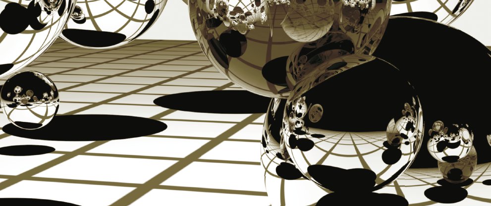

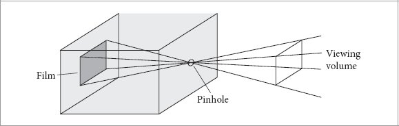


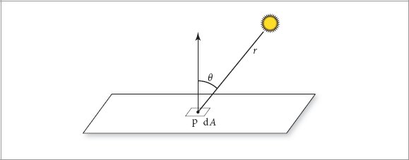
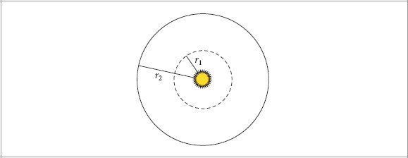


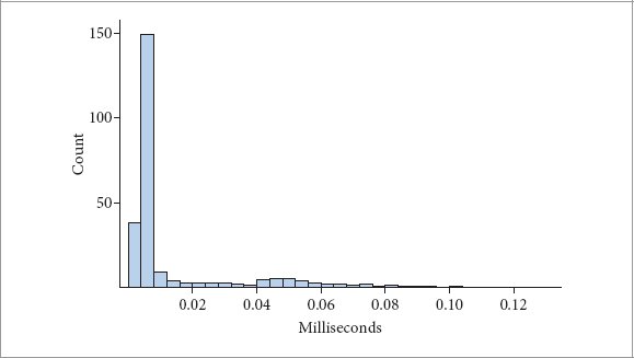
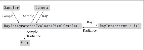


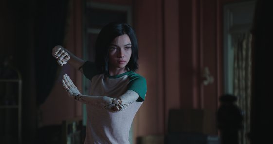
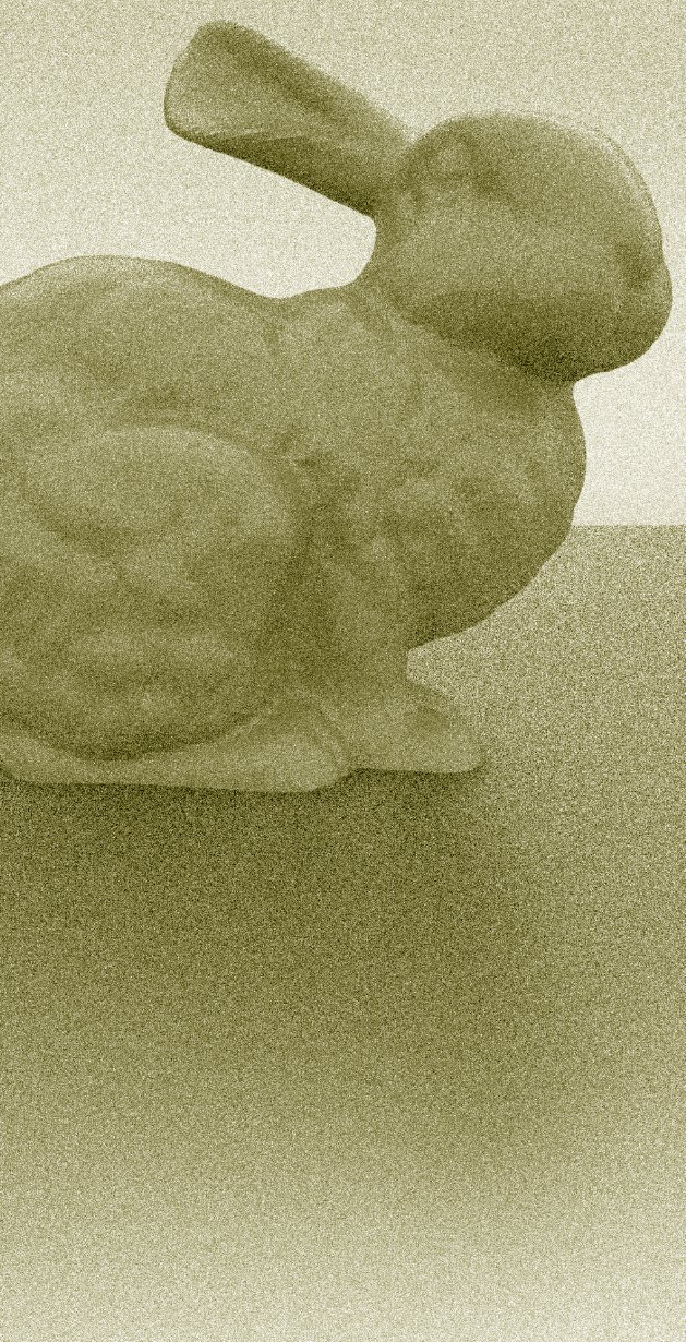
 , and the sum of probability ∑ pi is necessarily one. A random variable like this one that has the same probability for all potential values of it is said to be uniform. A function p(X) that gives a discrete random variable’s probability is termed a probability mass function (PMF), and so we could equivalently write
  in this case.


 , since two of the six possibilities are less than or equal to 2.


 . Given a supply of independent uniform random variables Xi ∈ [a, b], the Monte Carlo estimator says that the expected value of the estimator


 , then the sample variance is
 can be computed (for example, using a large number of samples), then the mean squared error can be estimated by


 , where vi is the fractional volume of stratum i (vi ∈ (0, 1]).
 . This shows that the variance of the overall estimator is


 , which is plotted in


 , and that wi(x) = 0 if pi(x) = 0.)
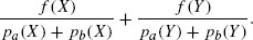
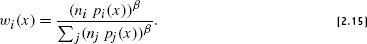
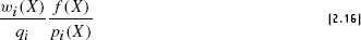


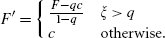
 . The corresponding PMF is shown in

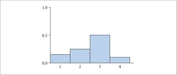

 .
.
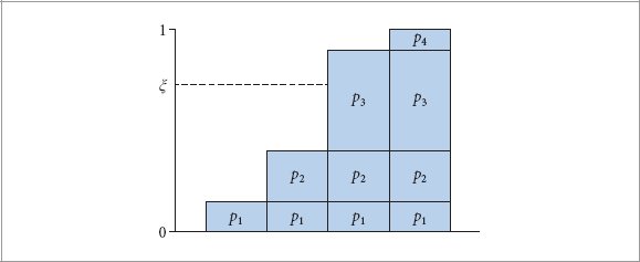
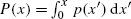 .
.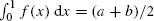 , which gives the normalization constant 2/(a + b) to define its PDF,


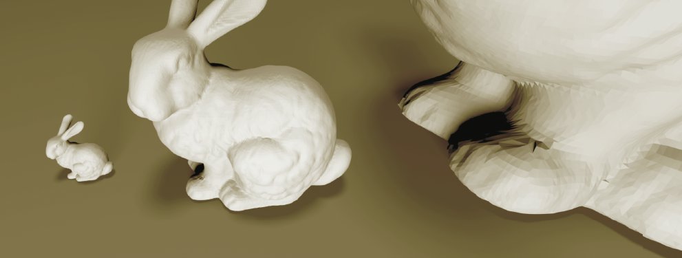

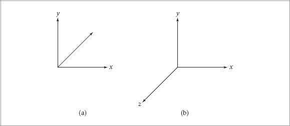


 is the normalized version of v. Before getting to normalization, we will start with computing vectors’ lengths.


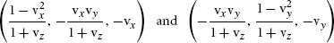


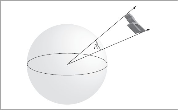

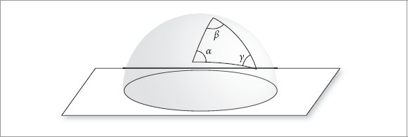


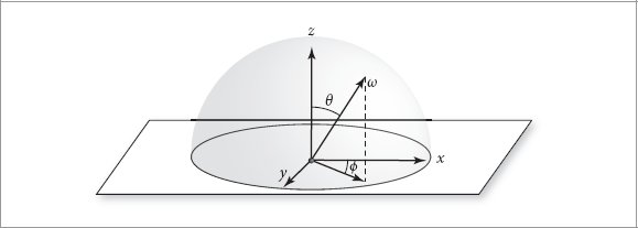

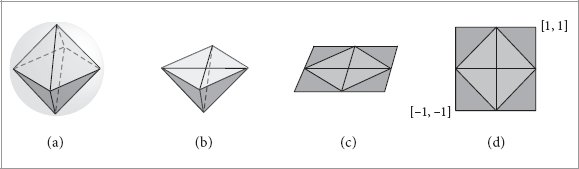


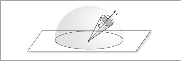
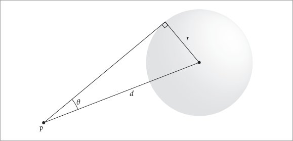
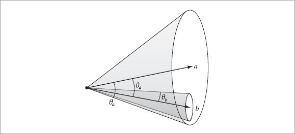

 . These four-vectors of three si values and a zero or one are called the homogeneous representations of the point and the vector. The fourth coordinate of the homogeneous representation is sometimes called the weight. For a point, its value can be any scalar other than zero: the homogeneous points [1, 3, −2, 1] and [−2, −6, 4, −2] describe the same Cartesian point (1, 3, −2). Converting homogeneous points into ordinary points entails dividing the first three components by the weight:

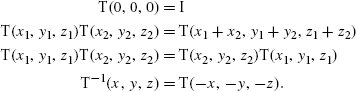
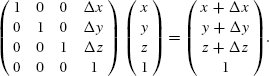


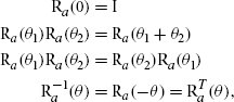
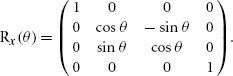


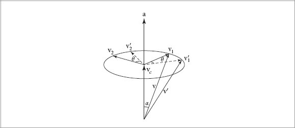

 , the absolute value of at least one pair of matching coordinates must then both be less than 0.72, assuming the vectors are normalized. In this way, a loss of accuracy is avoided when the reflection direction is nearly parallel to either


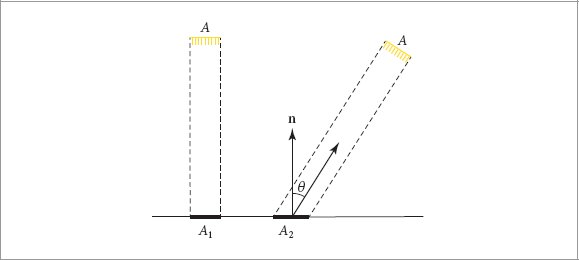


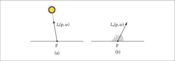


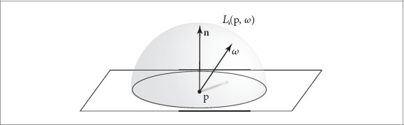


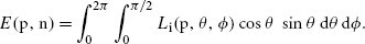
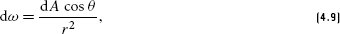


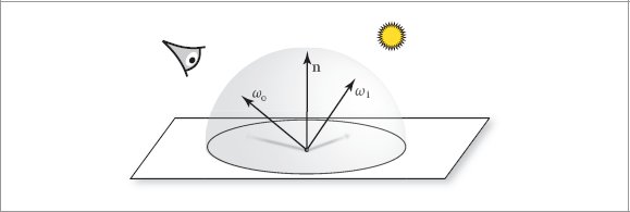
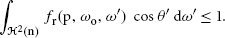


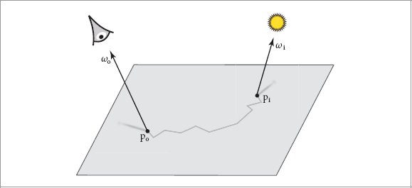

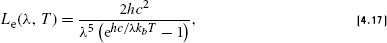
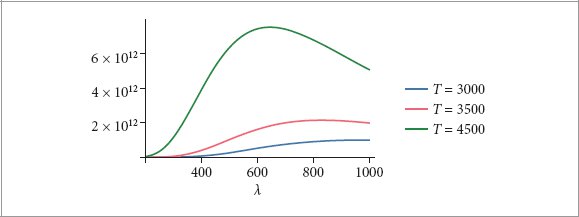


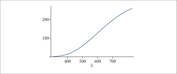
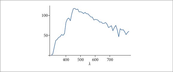


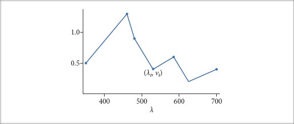

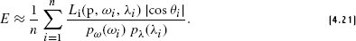
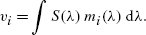
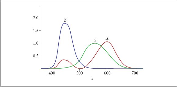

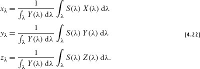
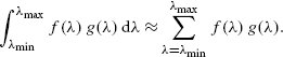
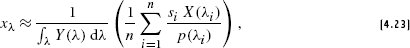


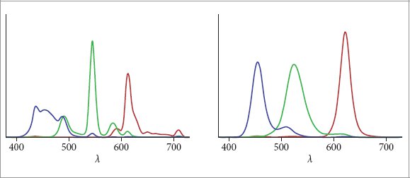
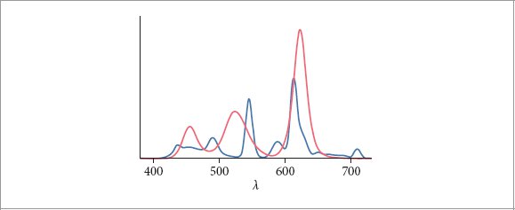
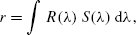
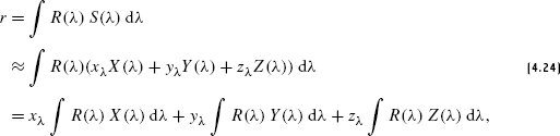
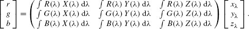
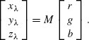
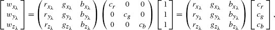
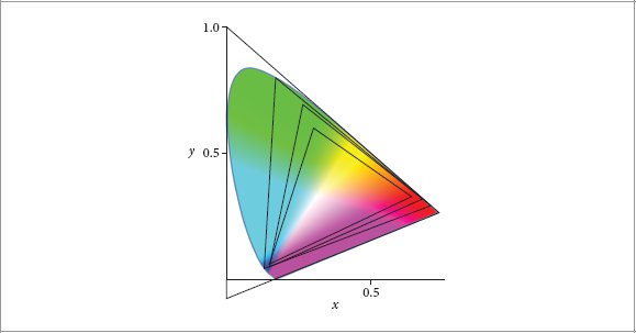
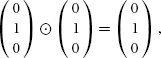
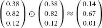

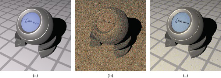
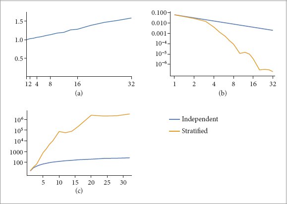
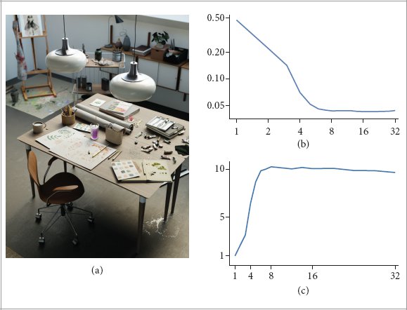
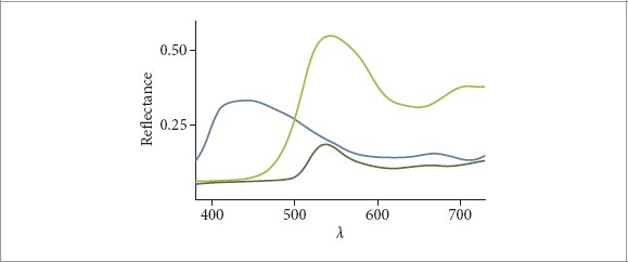

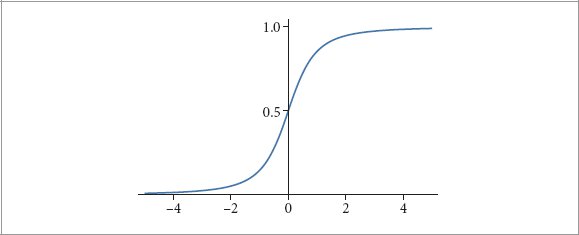

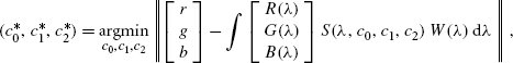
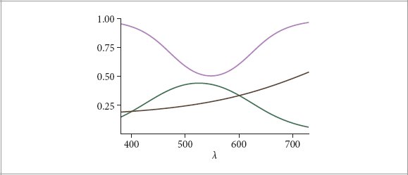
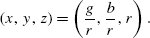
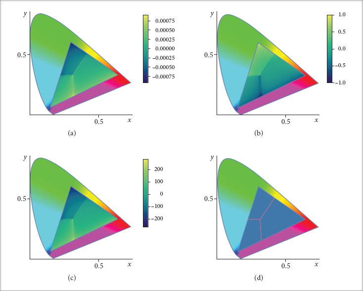
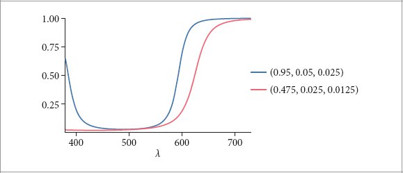
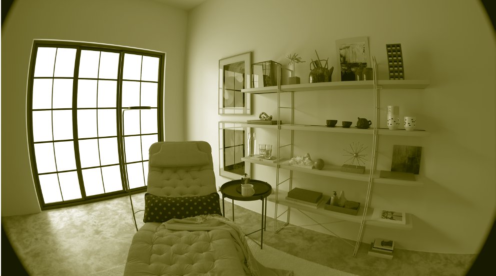
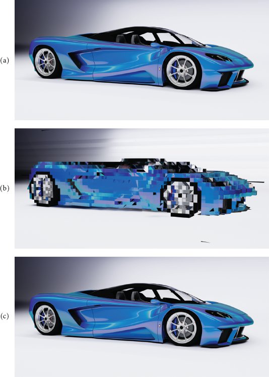
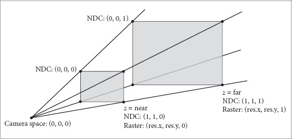

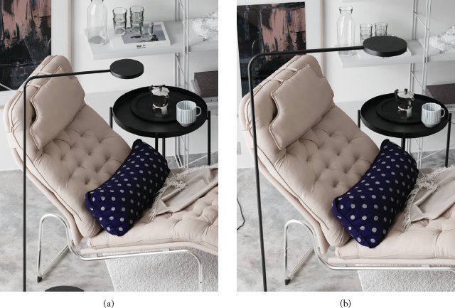
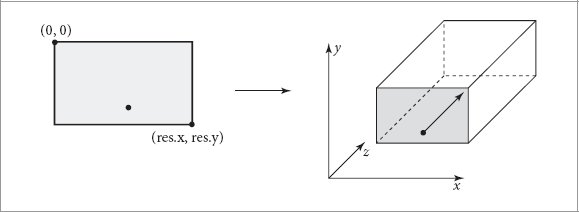
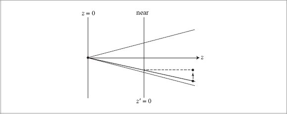

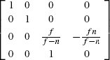

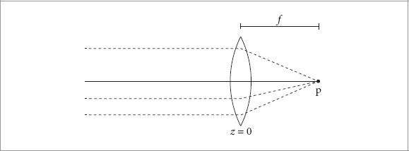
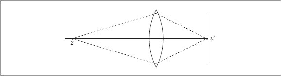
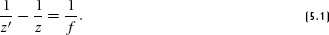
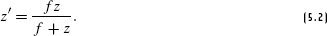
 . Given another point at depth z, the Gaussian lens equation gives the distance z′ that the lens focuses the point to. This point is either in front of or behind the film plane;
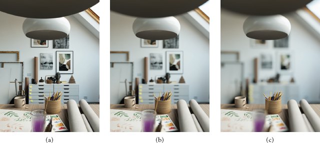
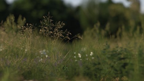
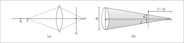
 .
.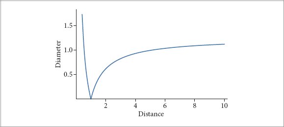
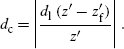
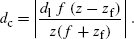
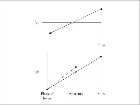
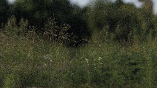
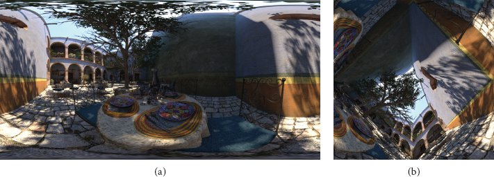
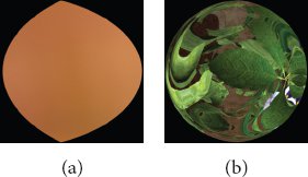


 ,
,  —and the imaging ratio as parameters. It also takes the color space requested by the user for the final output RGB values as well as the spectrum of an illuminant that specifies what color to consider to be white in the scene; together, these will make it possible to convert spectral energy to RGB as measured by the sensor and then to RGB in the output color space.
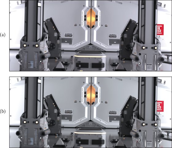
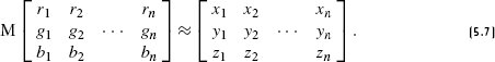
 for a tristimulus color space. It returns a triplet of color coefficients ci given by
 is a spectral matching function. Under the assumption that the second matching function
  generally corresponds to luminance or at least something green, the color that causes the greatest response by the human visual system, the returned color triplet is normalized by
  . In this way, the linear least squares fit at least roughly weights each RGB/XYZ pair according to visual importance.
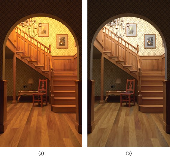
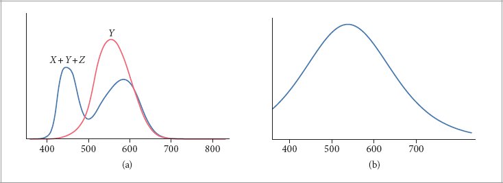
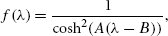
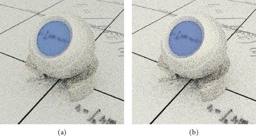
 with
with 
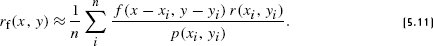
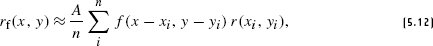
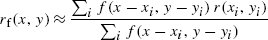
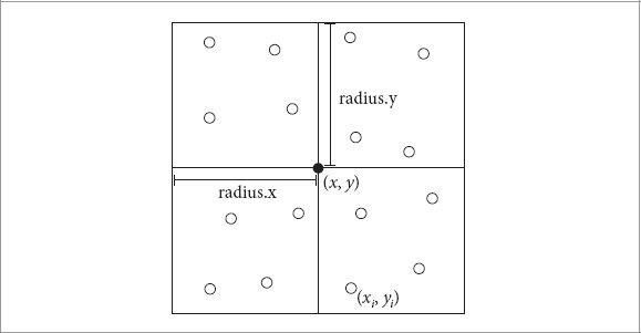


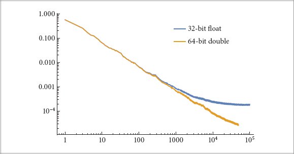
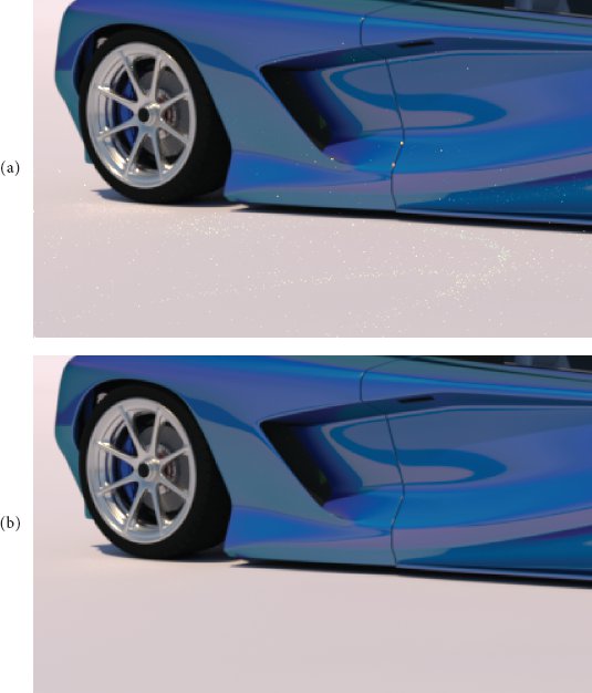

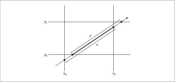
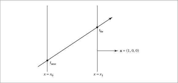
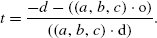

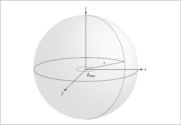
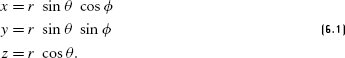
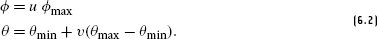
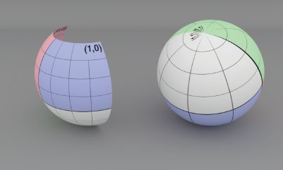
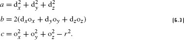
 approach that gives more accuracy; it is described in


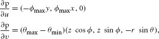
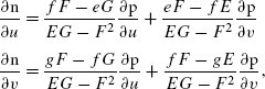
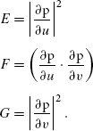

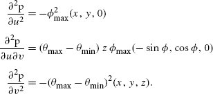
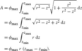

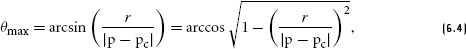
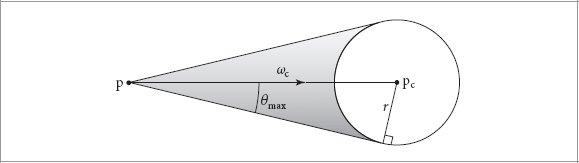
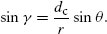

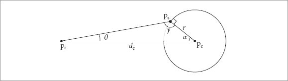
 , we can find
 .
.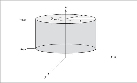
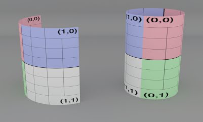
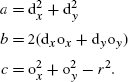
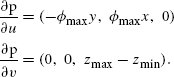
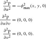
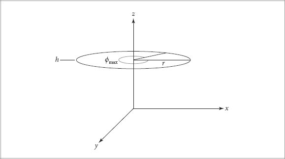
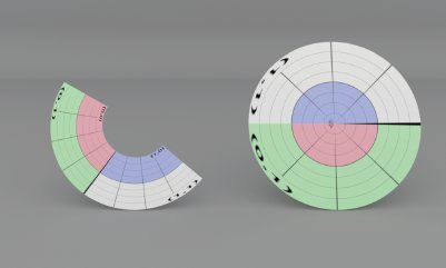
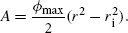


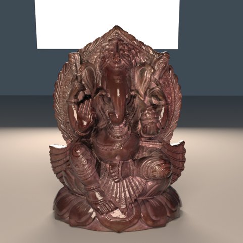
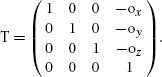
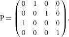
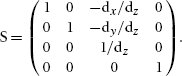
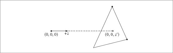
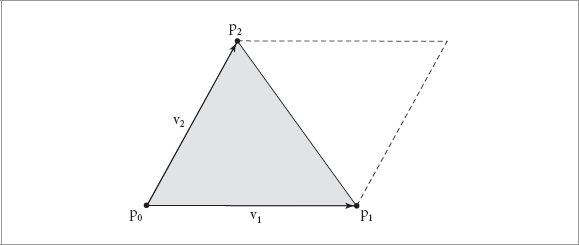

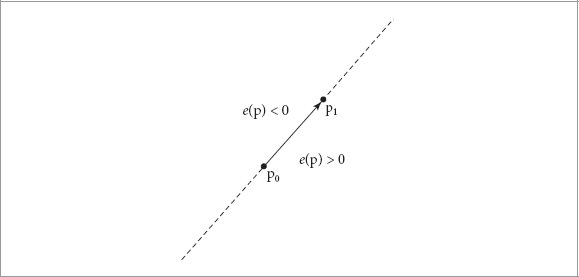

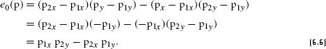
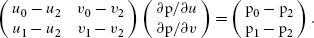
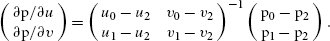


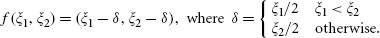
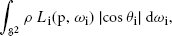
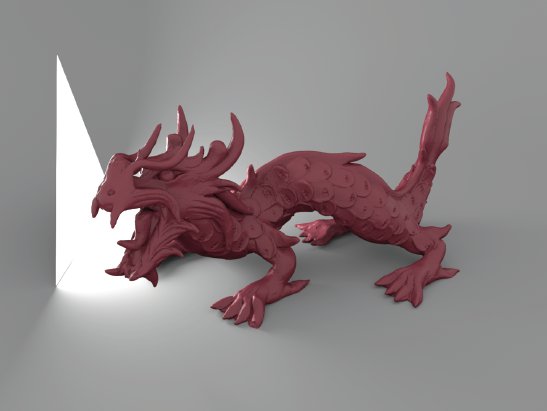
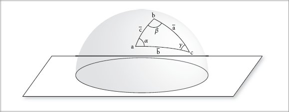
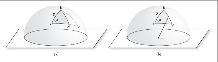

 in order to avoid needing to perform the subtraction.
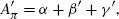
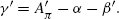
 to simplify notation, we have


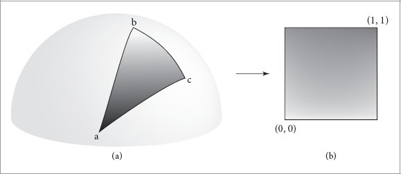
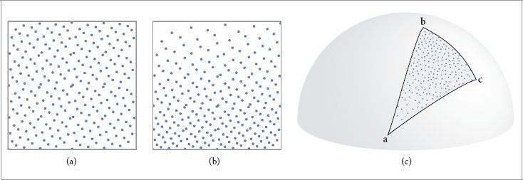
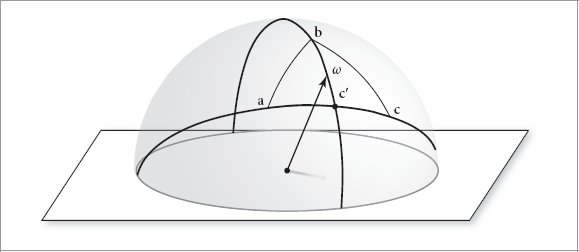

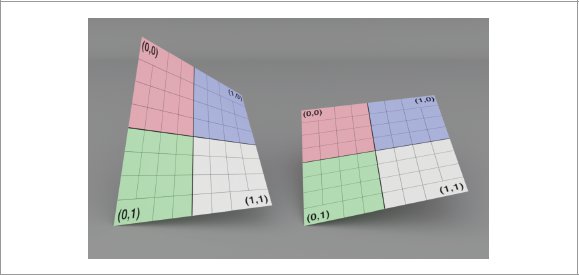
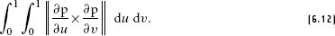
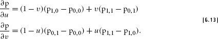
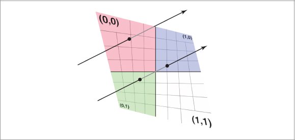
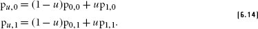
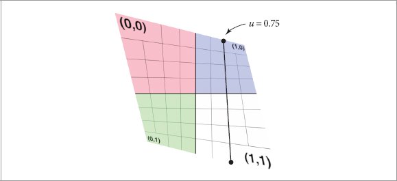
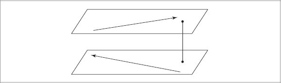
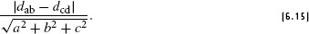
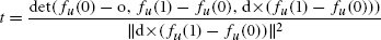
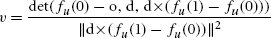
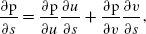
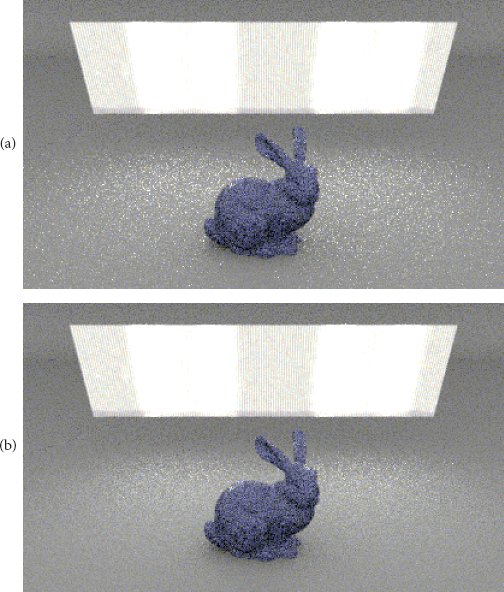
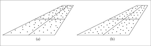
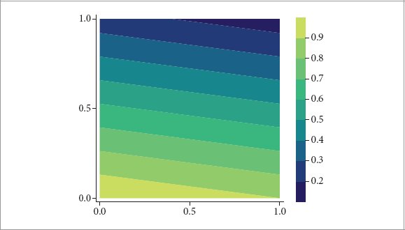


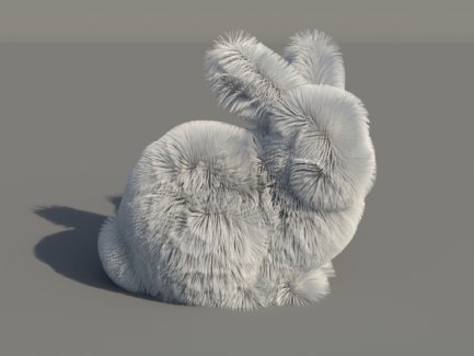
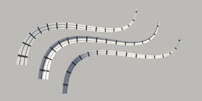
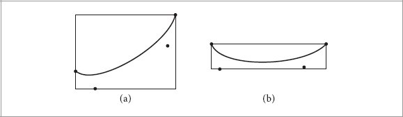


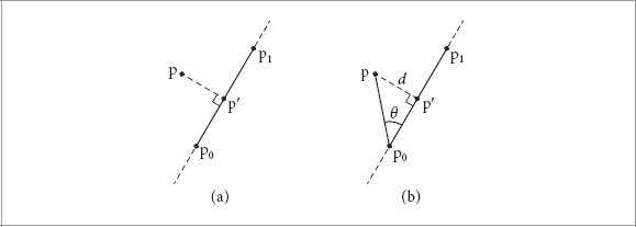
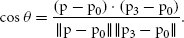
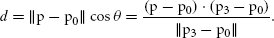
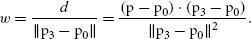
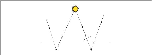


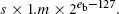


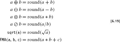

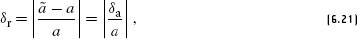


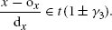

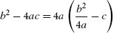
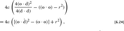
 is the ray’s normalized direction.
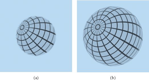

 is particularly problematic, since it is the difference of two positive values, so is susceptible to catastrophic cancellation.


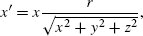
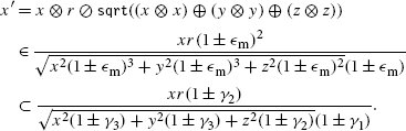
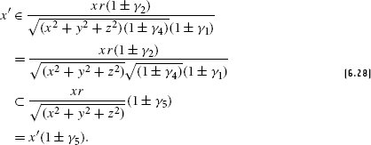

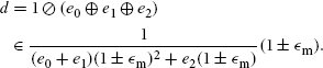
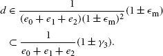
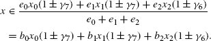


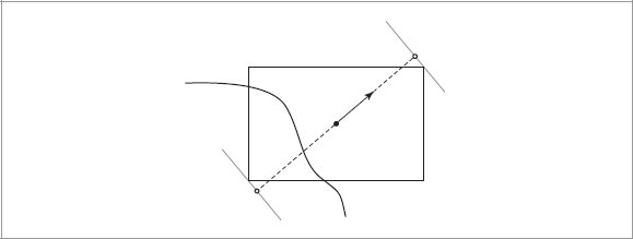


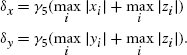


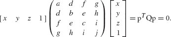
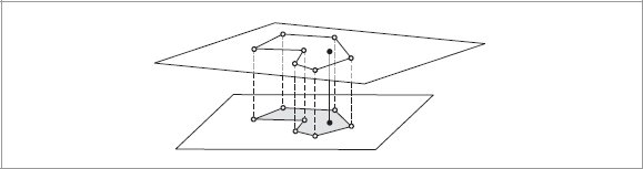
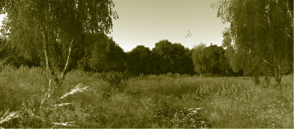
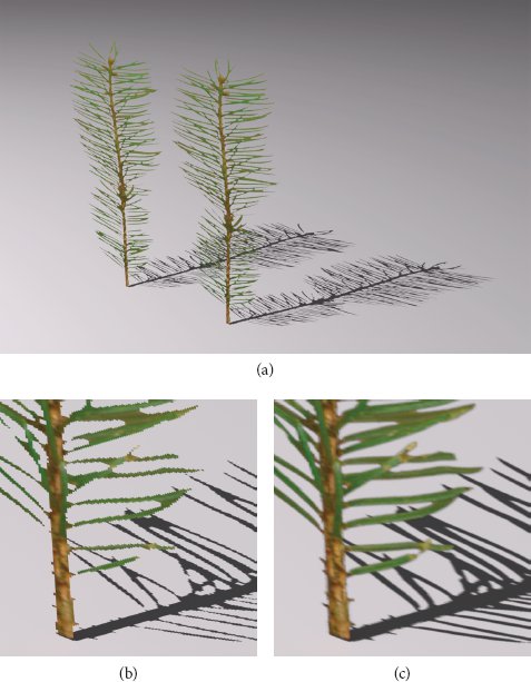
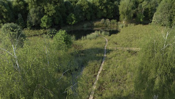
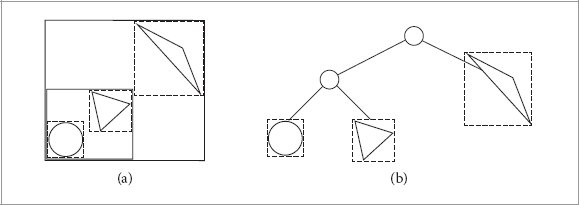
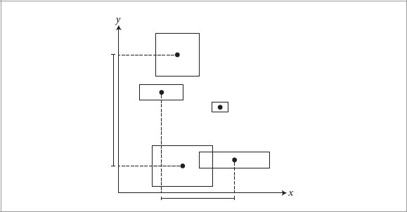
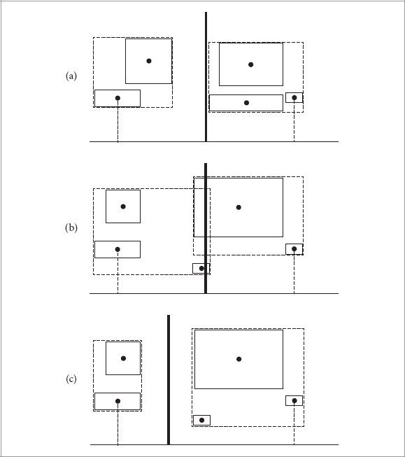

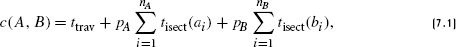
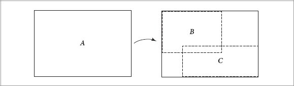

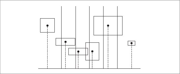

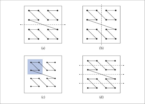
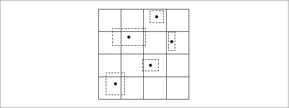

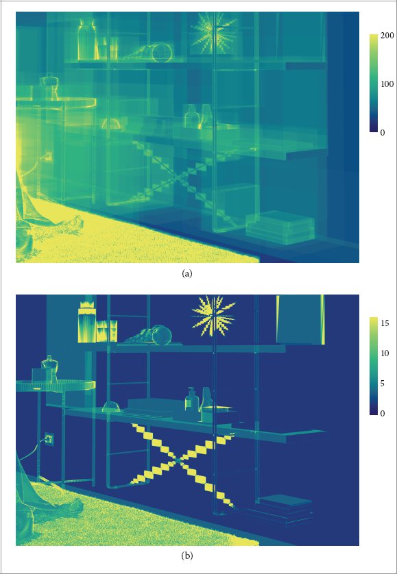
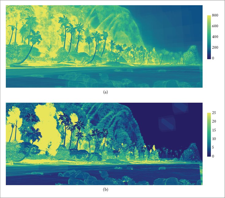
 that approximates the original function f. In this example,
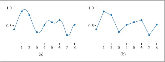
 that is an approximation to f (x). The sampling theorem, introduced in
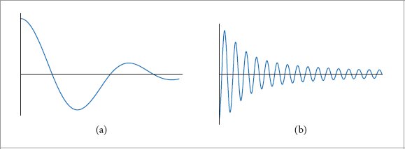
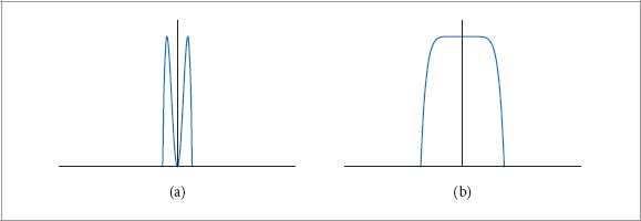

 .) For simplicity, here we will consider only even functions where f (−x) = f (x), in which case the Fourier transform of f has no imaginary terms. The new function F is a function of frequency, ω.
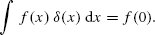


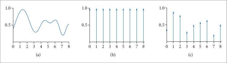
 , giving (c) an infinite sequence of scaled delta functions that represent its value at each sample point.
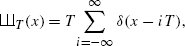
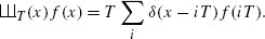
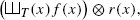
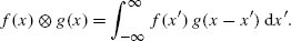
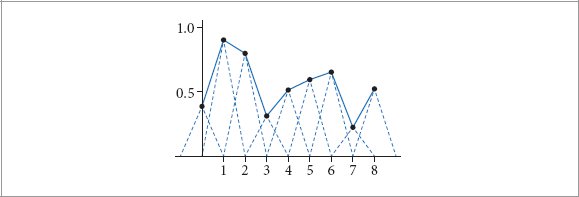
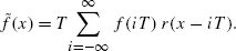


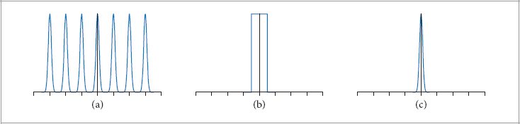

 with period T is a new shah function with period 1/T. This means that if the spacing between samples increases in the spatial domain, the sample spacing decreases in the frequency domain, pushing the copies of the spectrum F (ω) closer together. If the copies get too close together, they start to overlap.
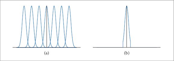
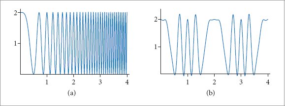


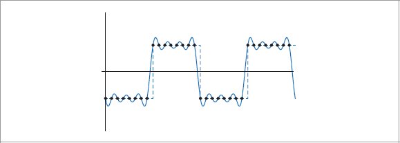
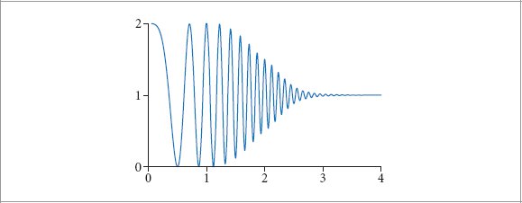
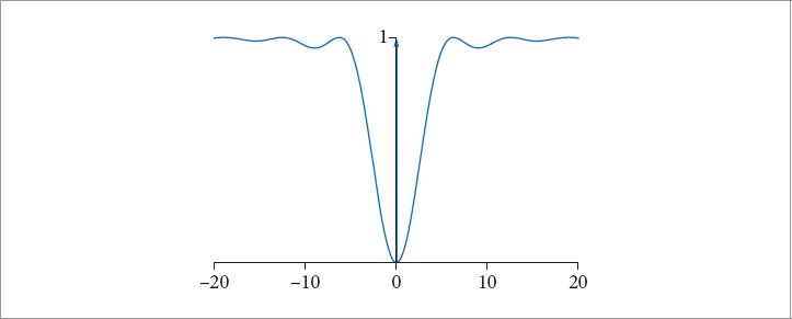
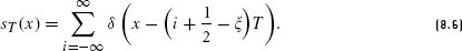

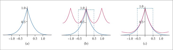
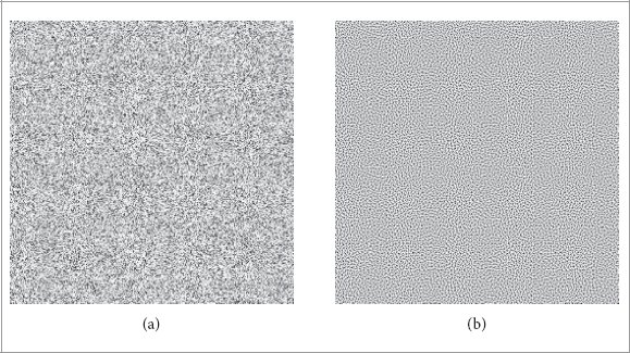

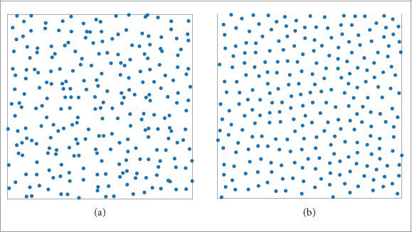
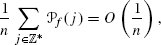
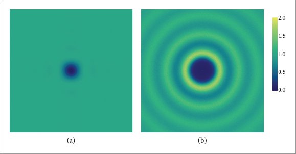
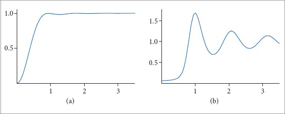
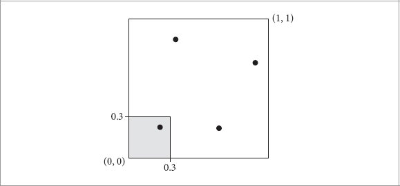


 . Another popular option for B is the set of all axis-aligned boxes, where the restriction that one corner be at the origin has been removed.

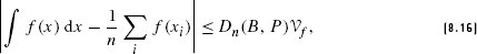
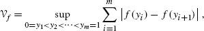
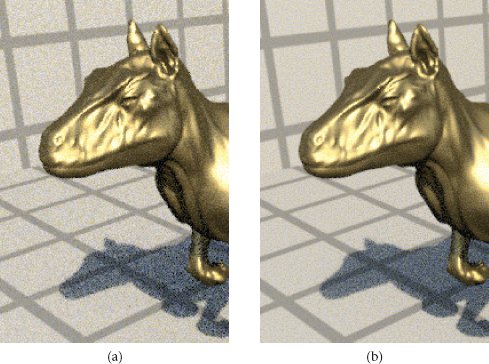
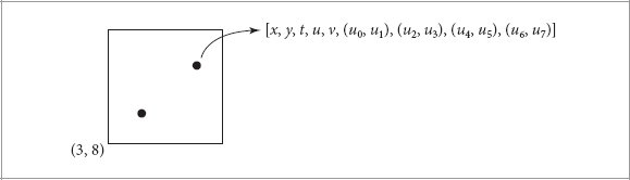
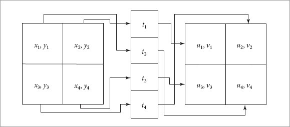
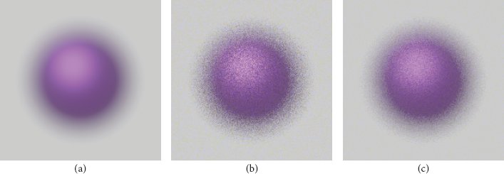
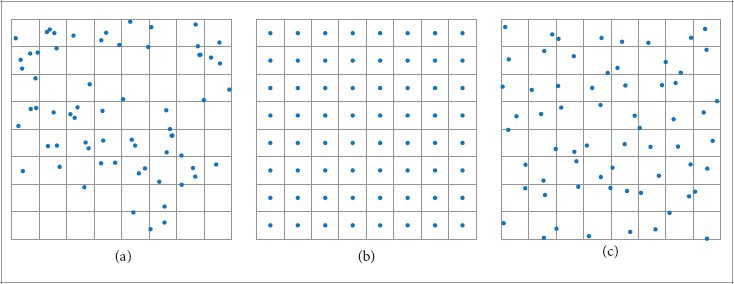
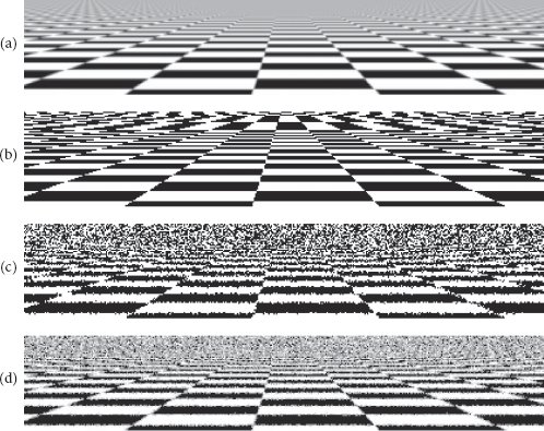
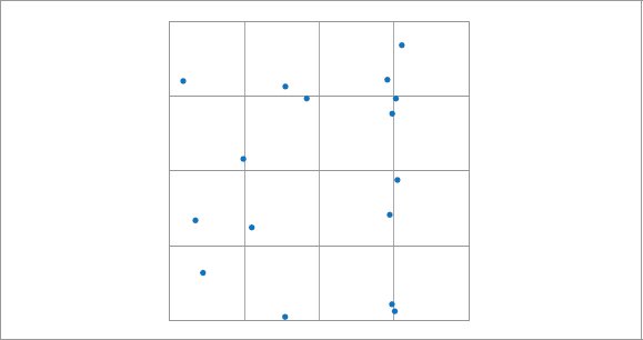
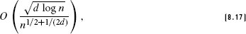
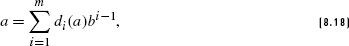
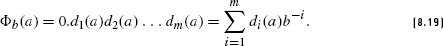

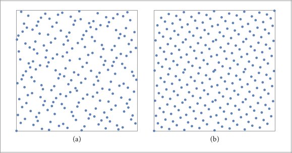
 for integer ki.)

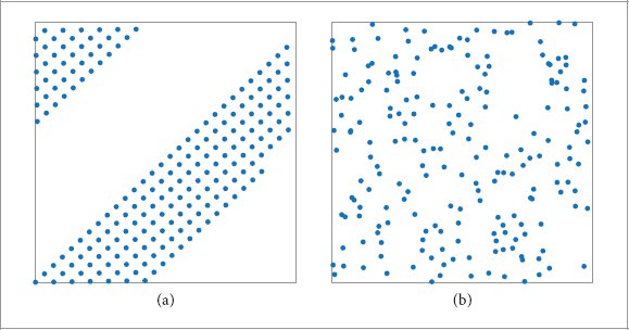

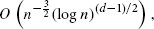
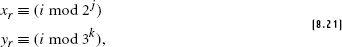
 are guaranteed to be stratified along either of the dimensions, whereas with the Halton sampler, all n are.)
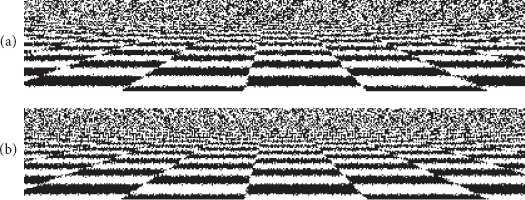
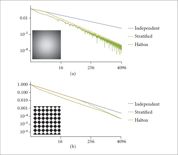
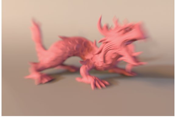
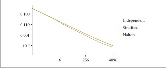
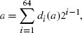


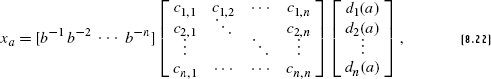
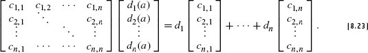
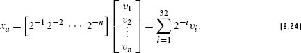
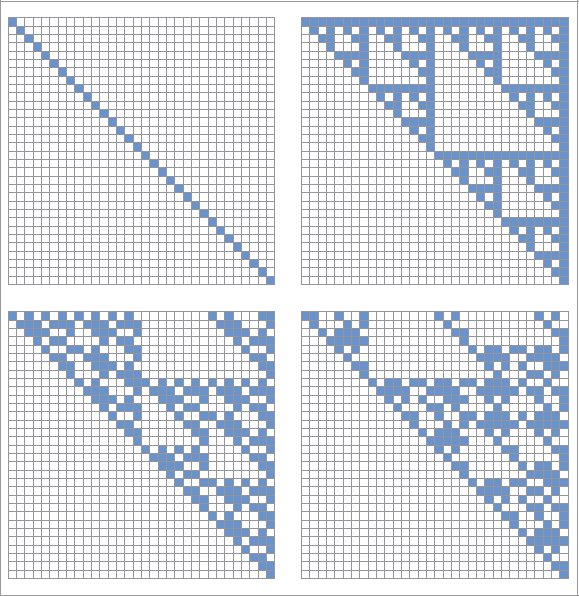
 ,
,  , 1) and (1,
  ,
,  ) and (
 (where li is a non-negative integer) satisfies this general stratification constraint. The set of elementary intervals in two dimensions, base 2, is defined as
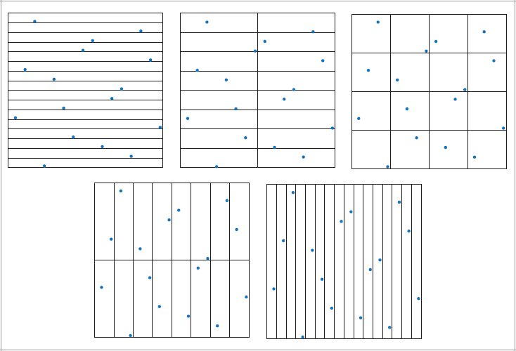
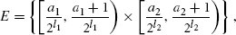
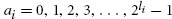 . One sample from each of the first

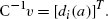
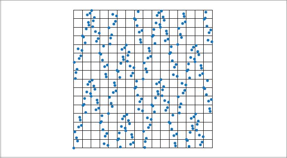
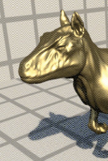
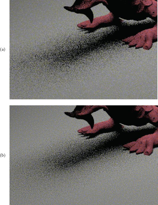
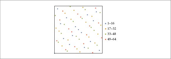
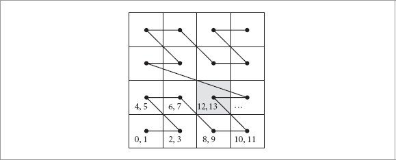
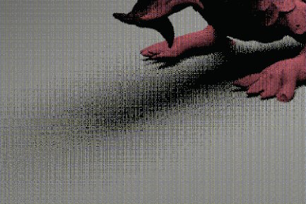
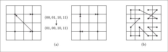

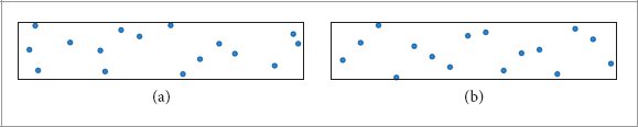
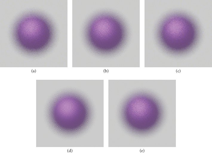
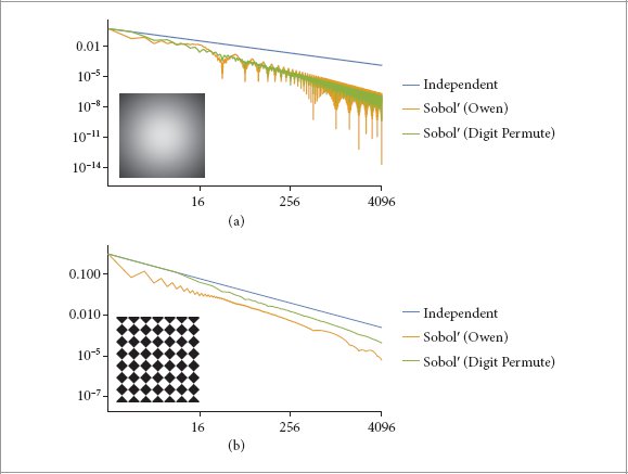
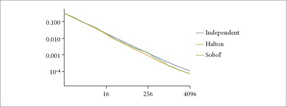
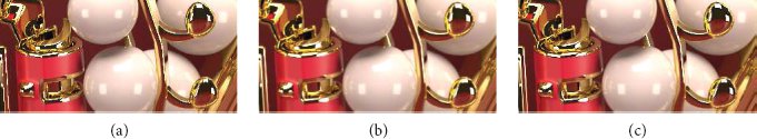
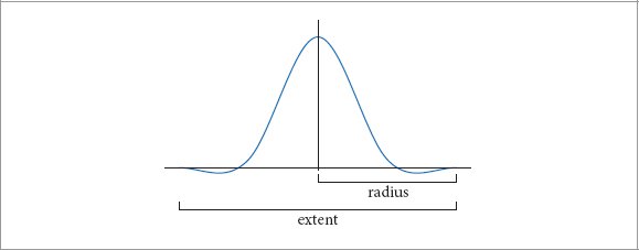
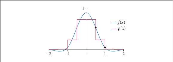
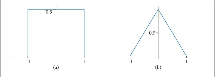
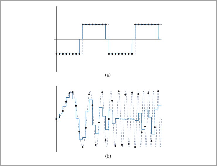
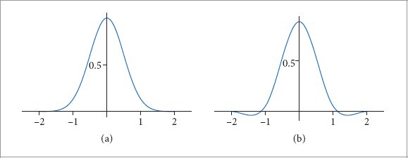
 and
and  , each with a width of 2. The Gaussian gives images that tend to be a bit blurry, while the negative lobes of the Mitchell filter help to accentuate and sharpen edges in final images.
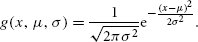

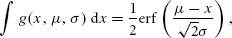
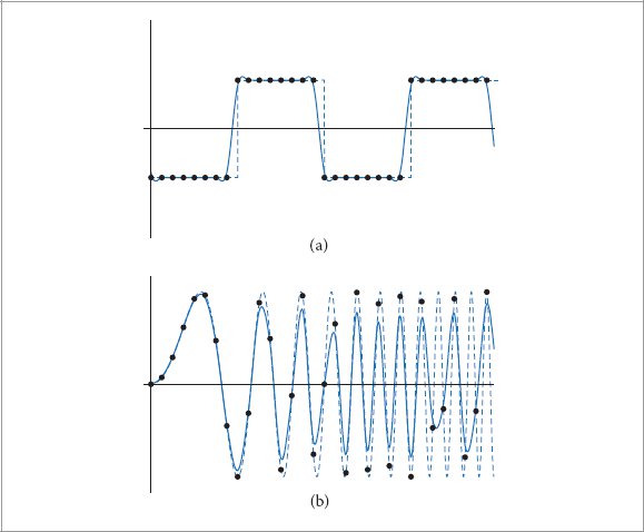
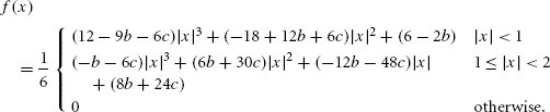
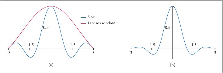

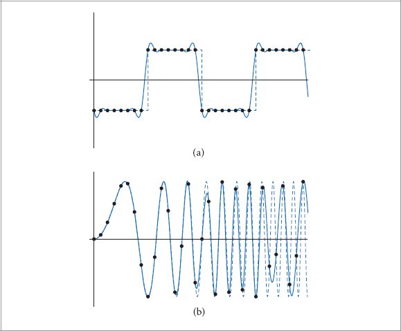
 .
.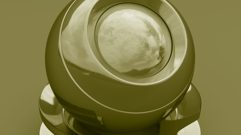
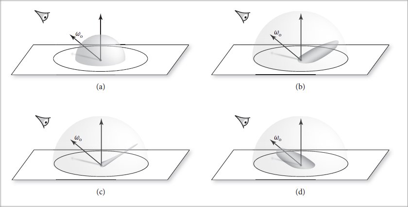
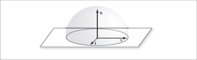
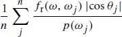

 so that the total integrated reflectance equals R.
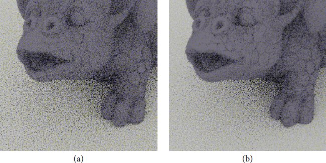
 compared to the size of objects rendered in
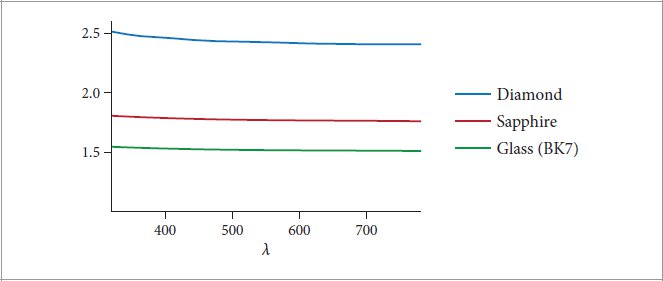
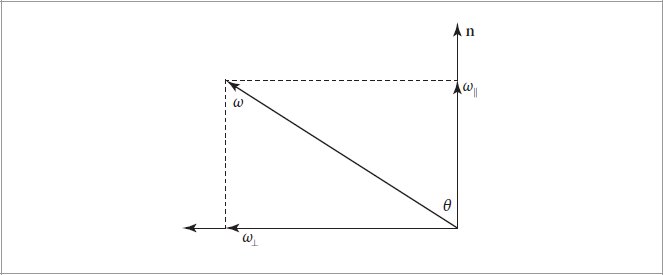
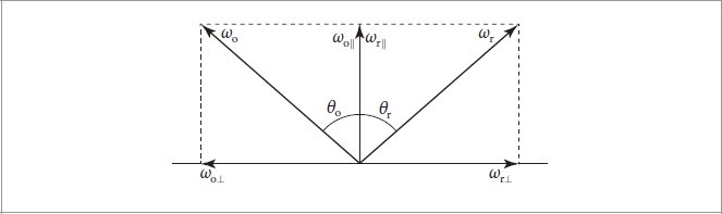
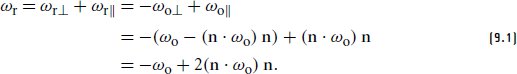


 specifies the proportional slowdown incurred when light passes through the interface. We will generally follow the convention that relevant laws and implementations are based on this relative quantity.
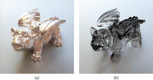
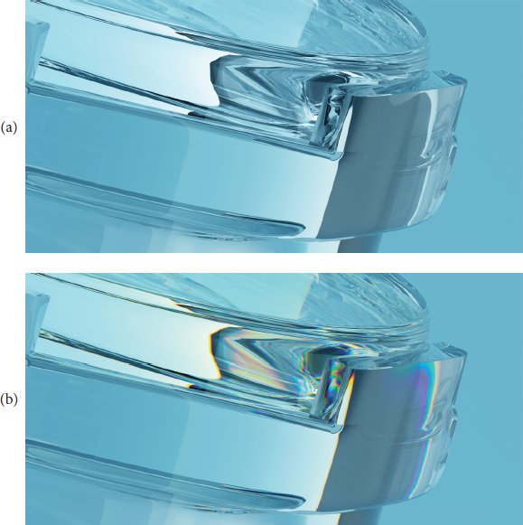
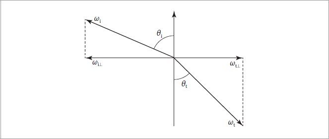
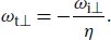
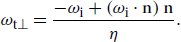

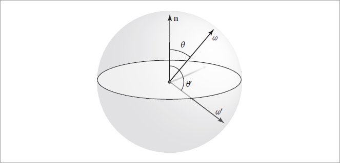
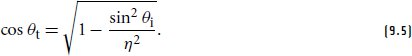
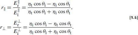
 matters, and we therefore prefer the equivalent expressions
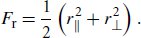
 obtained using complex division.
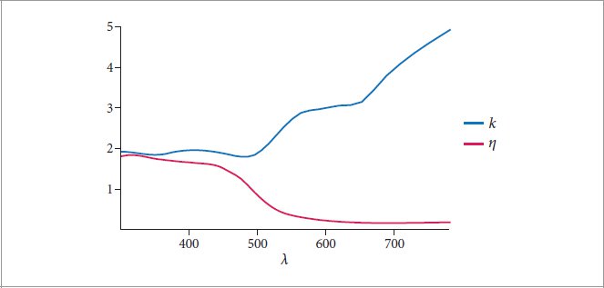
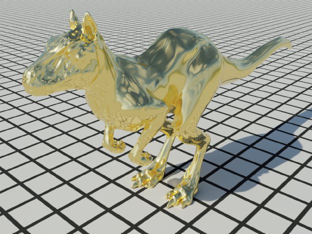


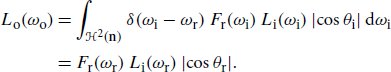

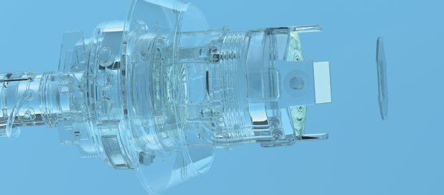
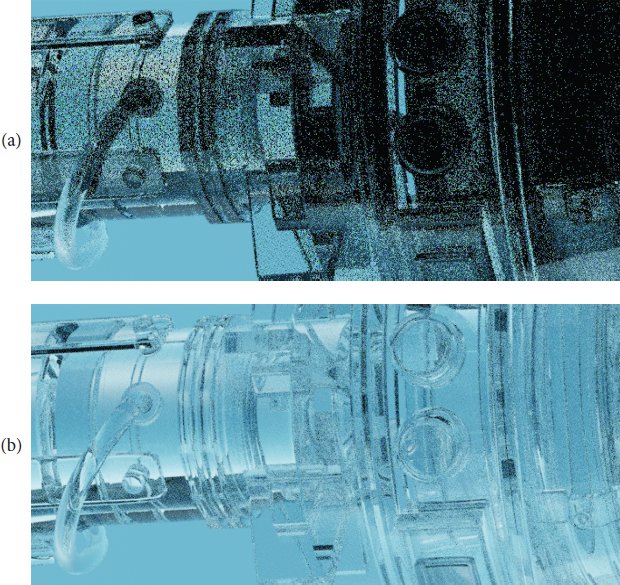
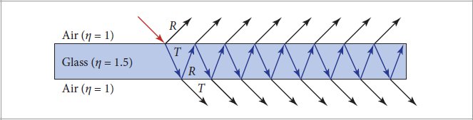

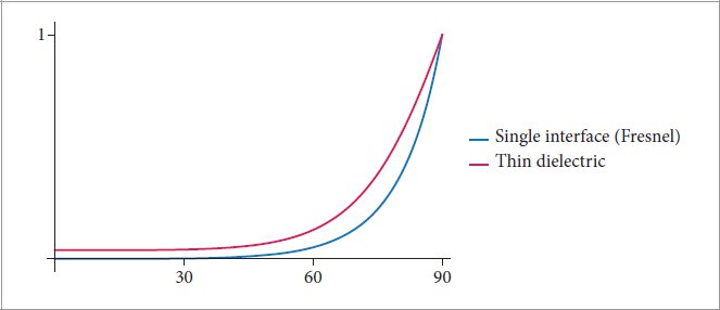
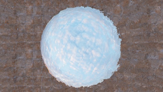
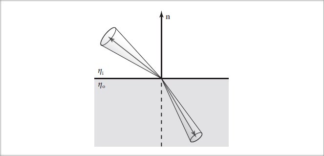

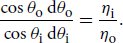
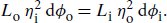
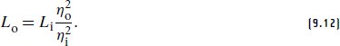

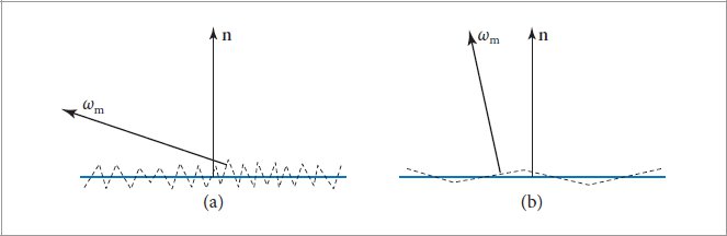
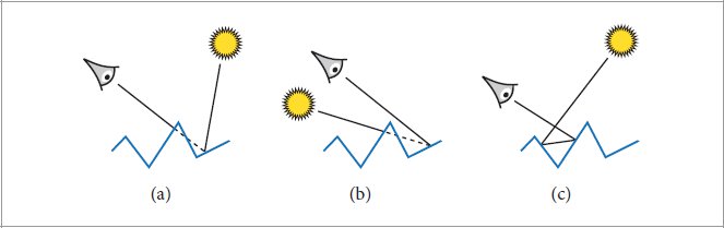


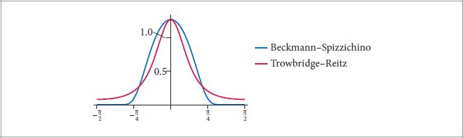
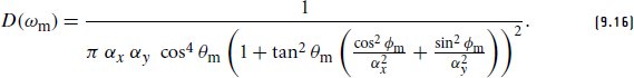
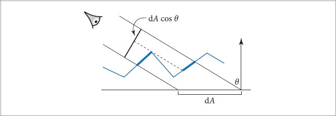

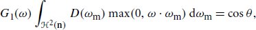

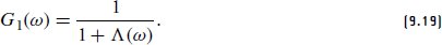


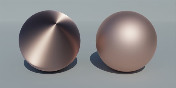
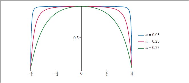

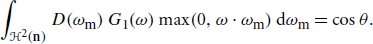


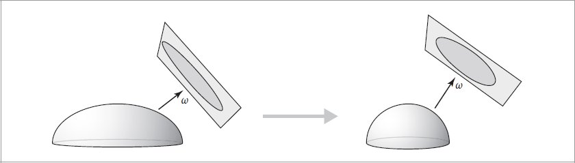
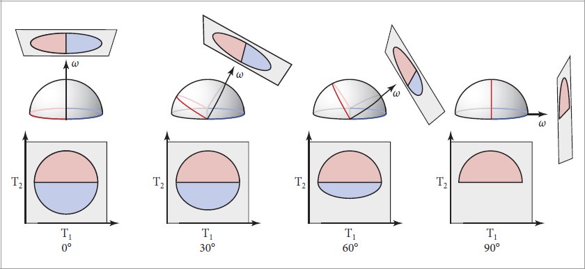
 specifies the maximum height. Due to non-perpendicular projection, this interval must now be reduced to [−h cos θ, h], which requires an affine transformation with scale
  and offset
  . The following fragment efficiently performs this transformation using the
  . This step encapsulates the process of intersecting the viewing ray with the random microstructure.
 , and that ωi is obtained from ωm and ωo using the law of specular reflection—that is,
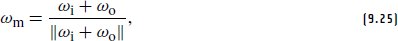

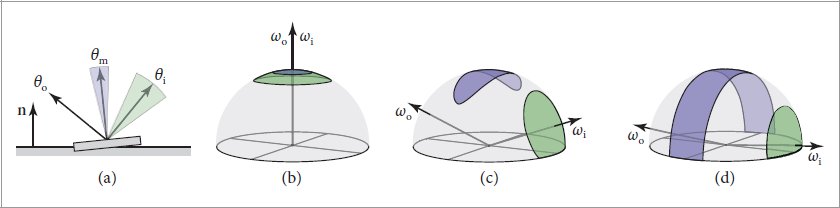
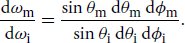
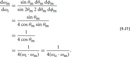

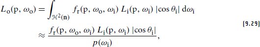


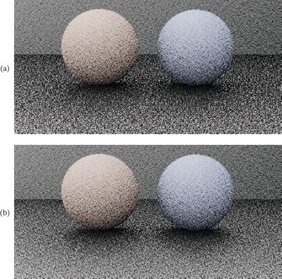
 .
.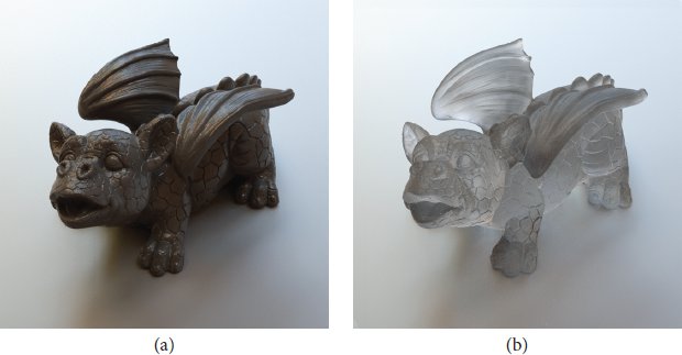


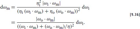


 with k = 1, … , n and use some kind of sensor (e.g., a photodiode) to record the reflected light scattered along a set of m outgoing directions
  with l = 1, … , m. These n × m measurements could be stored on disk and interpolated at runtime to approximate the BRDF at intermediate configurations (θi, ϕi, θo, ϕo). However, closer scrutiny of such an approach reveals several problems:
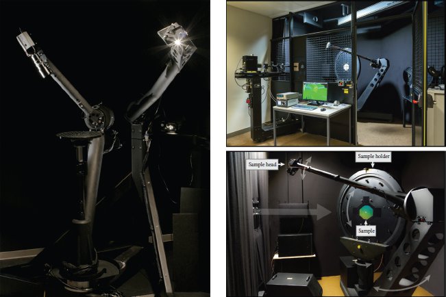
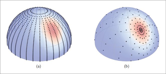
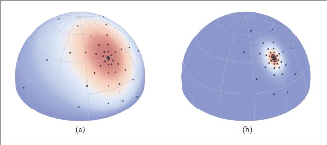

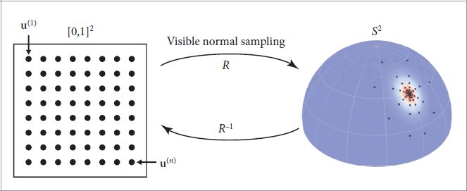
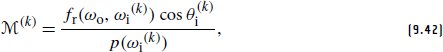
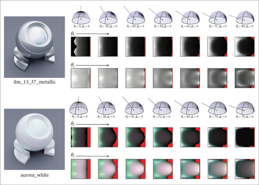

 and rearranging terms yields


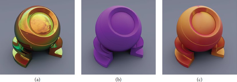
 parameterized by ωo = (θo, ϕo) in
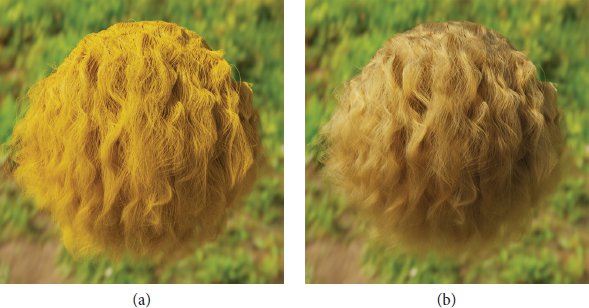
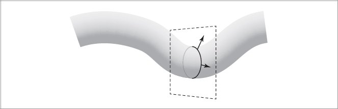
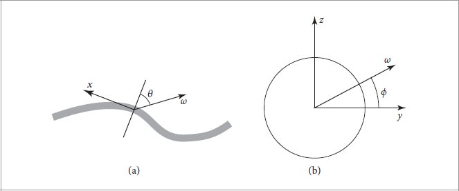
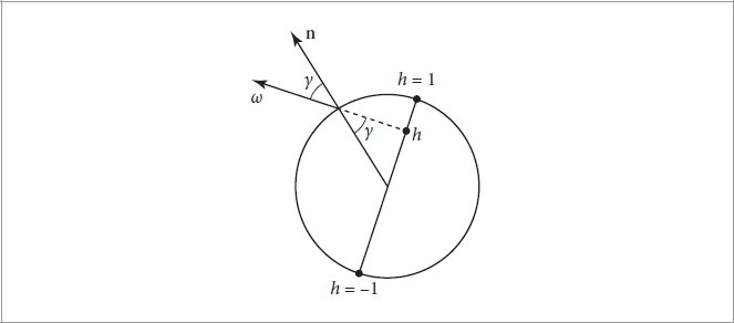
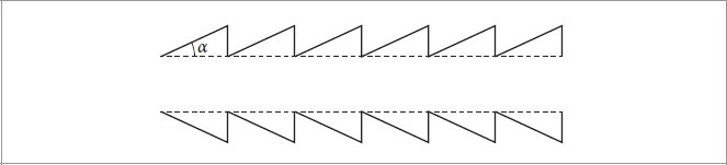
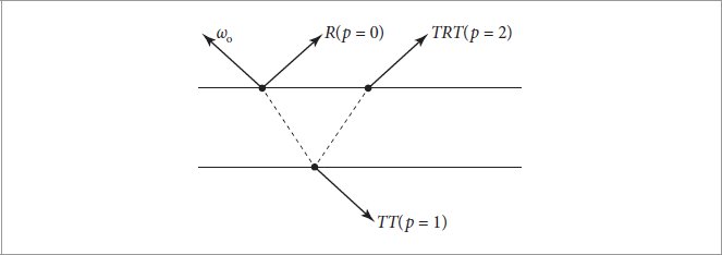
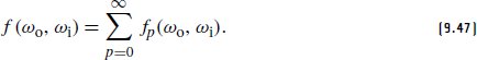

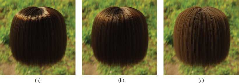

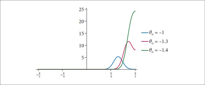
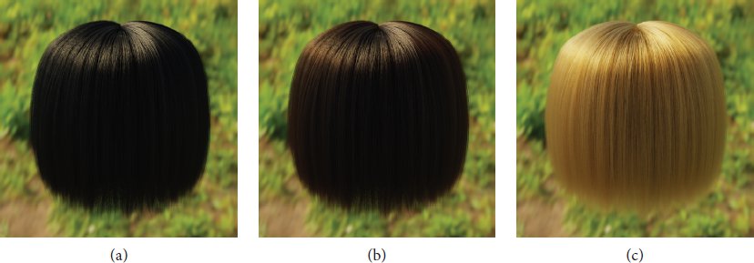
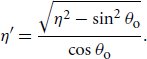
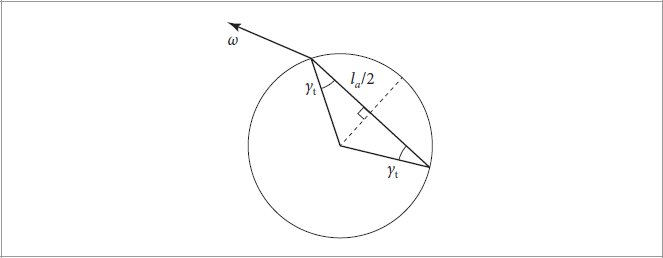


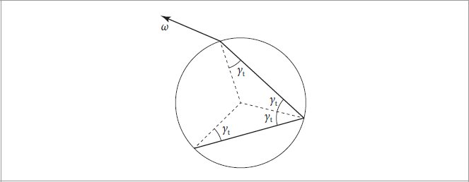
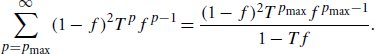
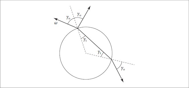
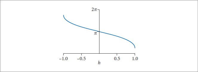
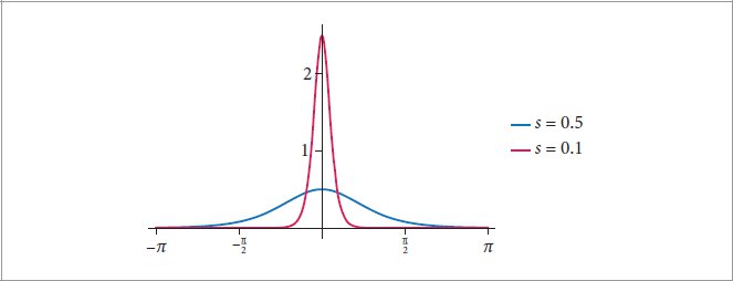
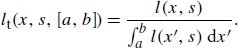
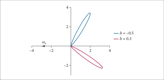
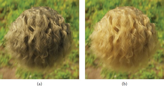
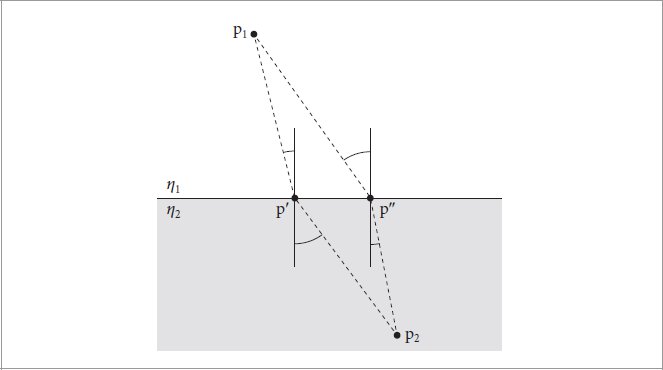
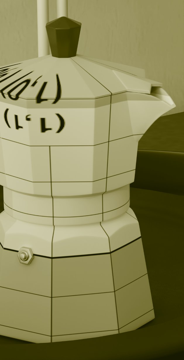
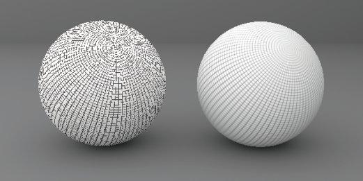
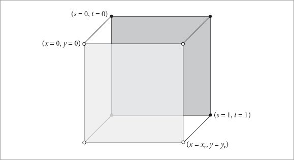
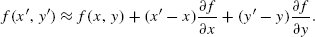
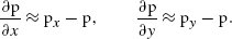
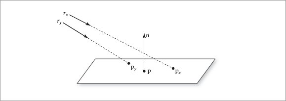
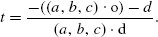
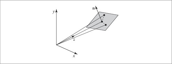
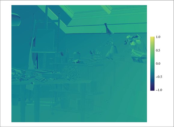

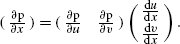

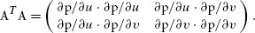


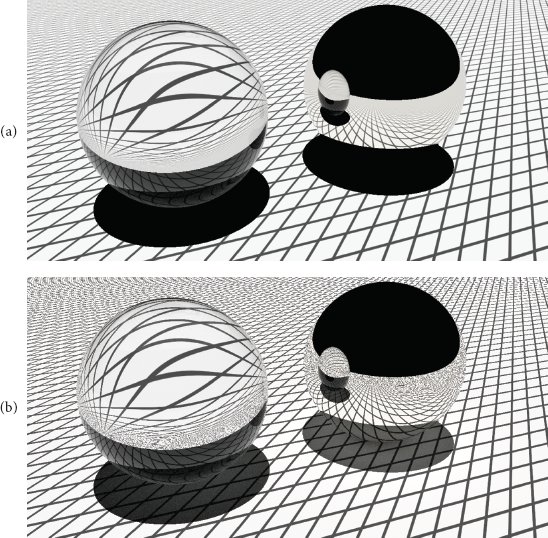
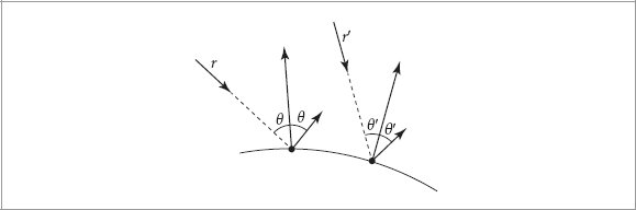

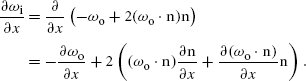
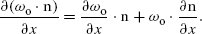
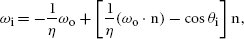

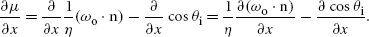
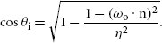
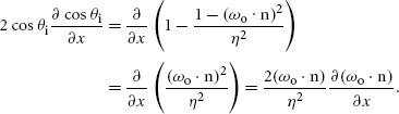
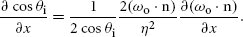


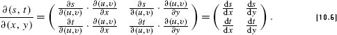


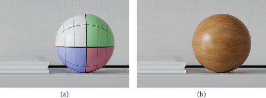
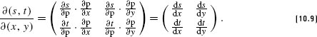
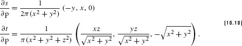
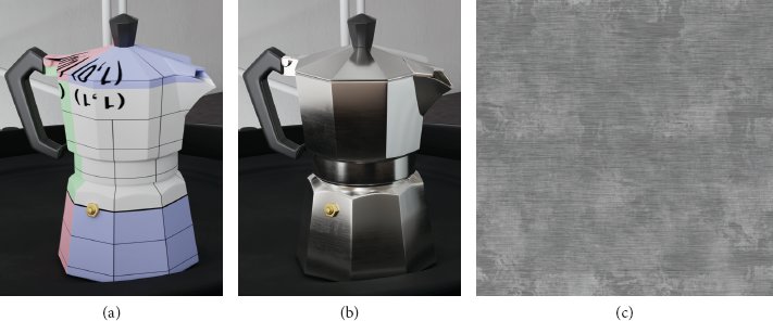
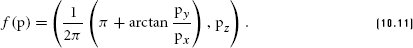

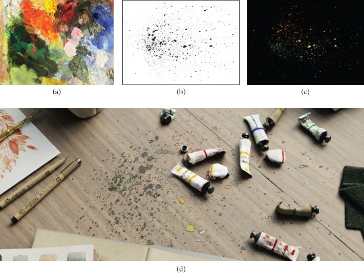
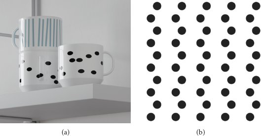
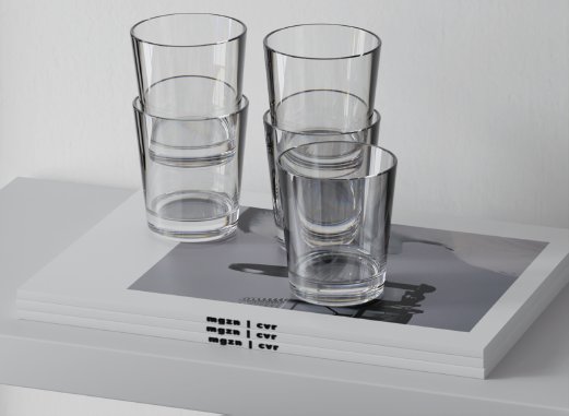
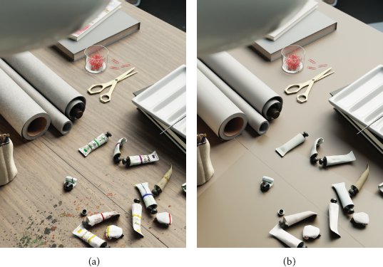

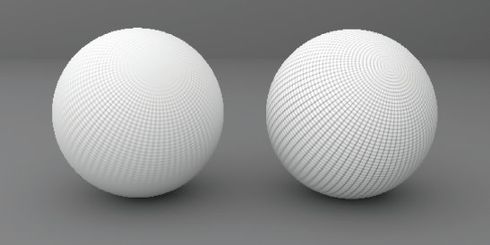
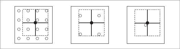
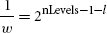


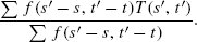

 .
.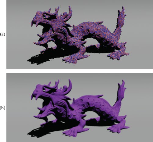
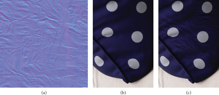

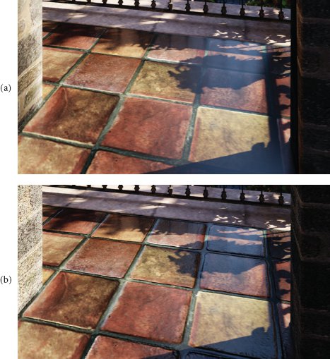
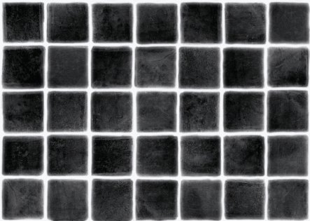

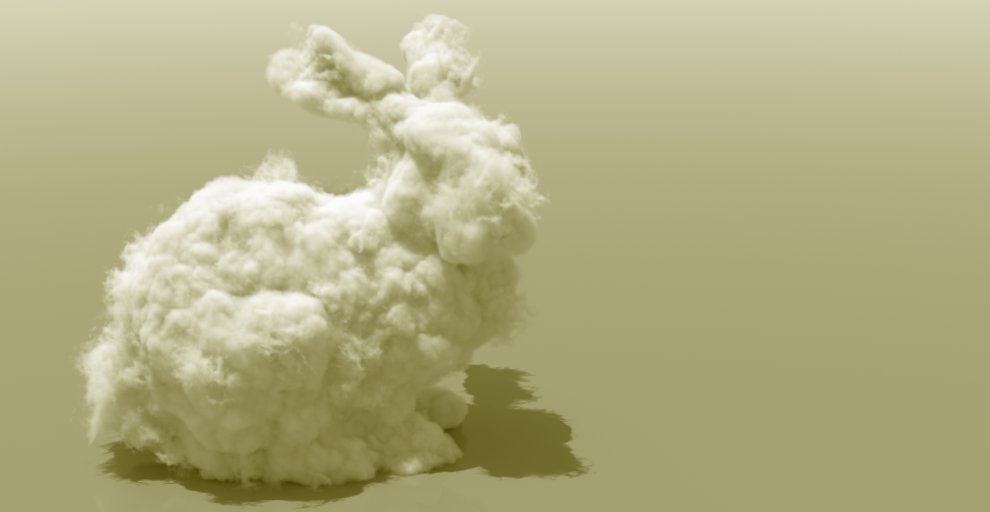
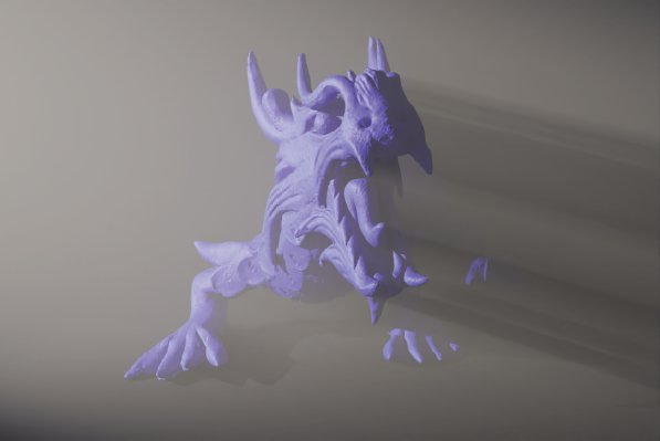
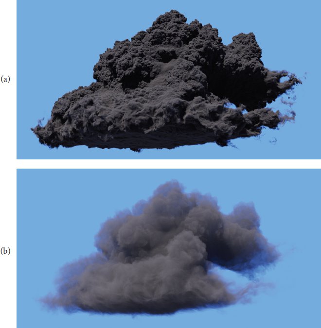
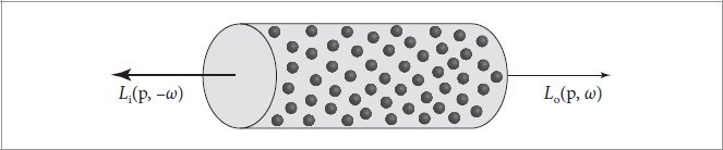
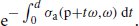

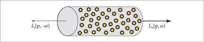
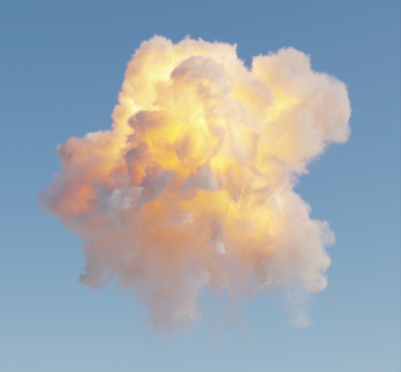
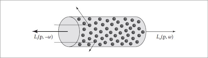
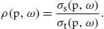
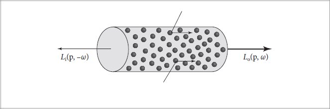
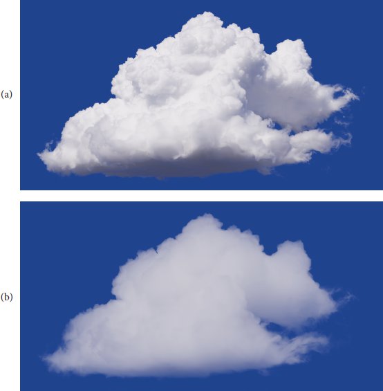
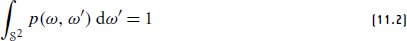


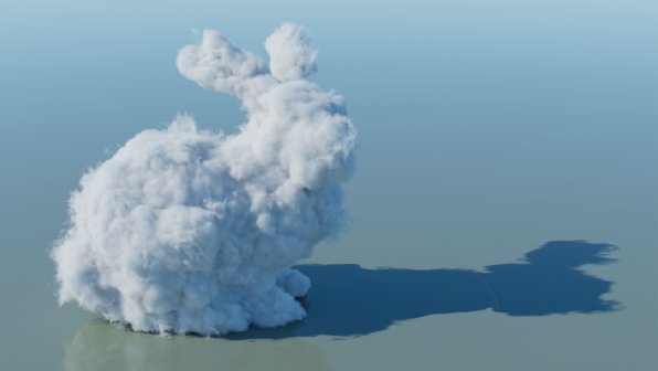


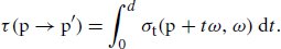


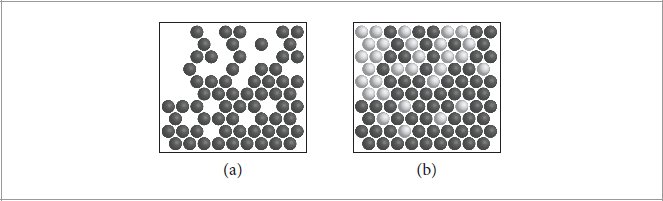


 is
is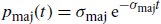


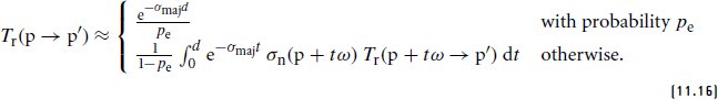
 . Then, the first case of
  . (This can be seen using pmaj’s cumulative distribution function (CDF),
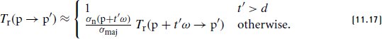
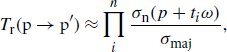
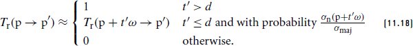
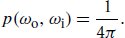

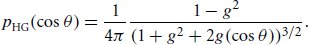

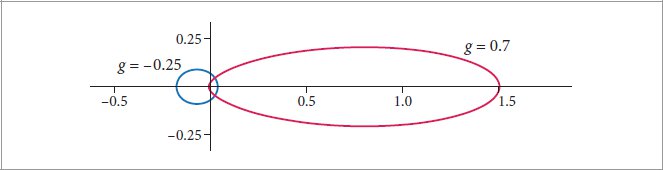
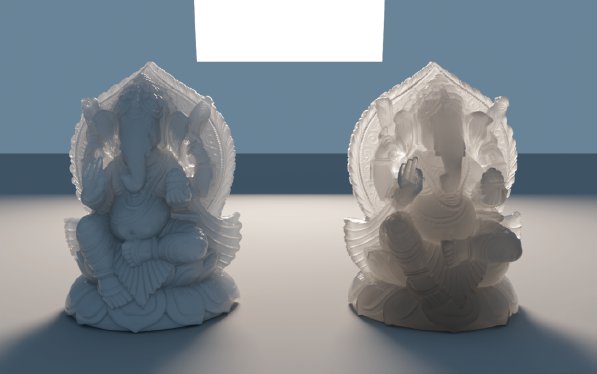
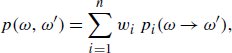
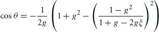
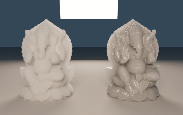

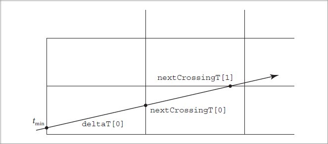
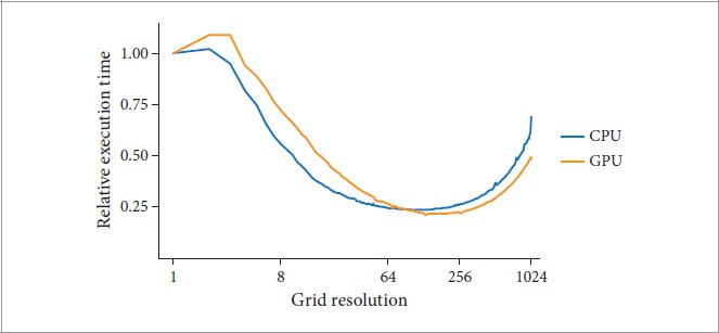
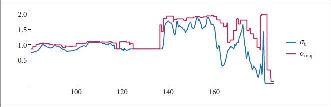
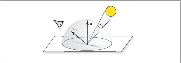
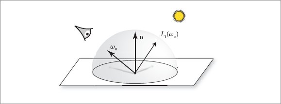
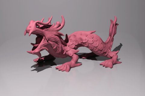
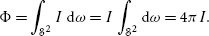
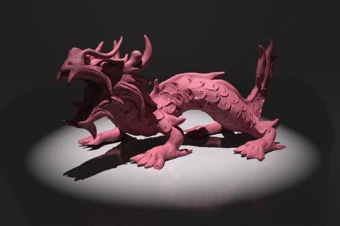
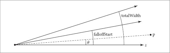
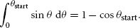

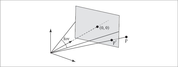
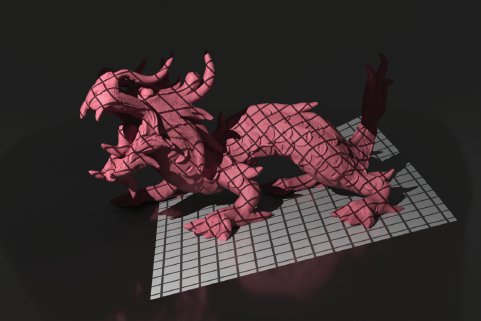
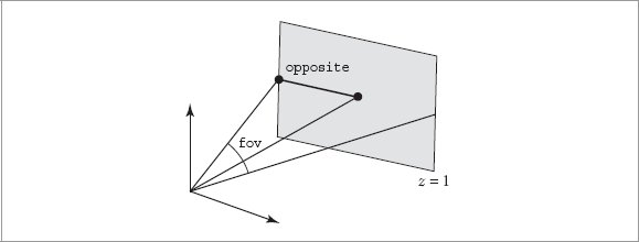
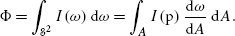
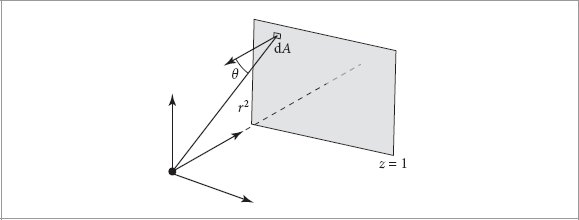

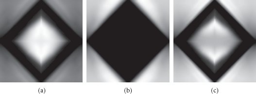
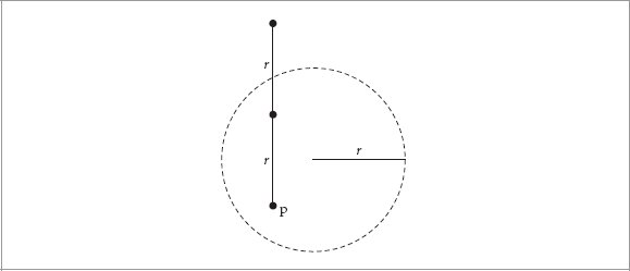
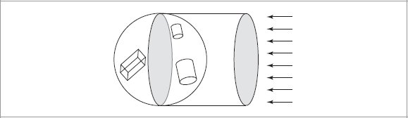
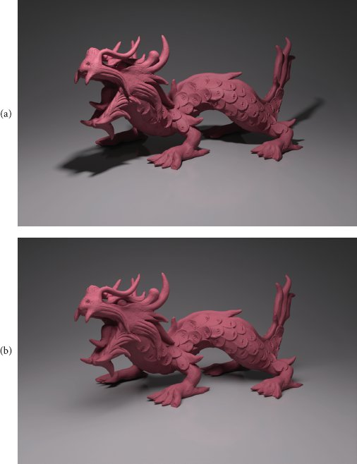
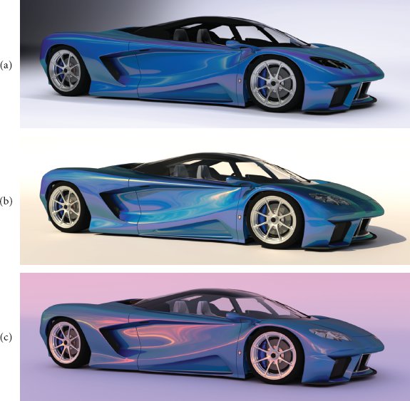
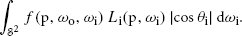
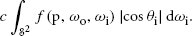
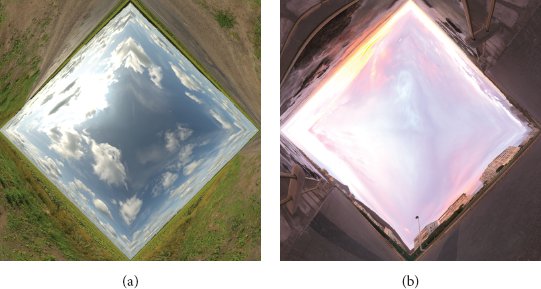
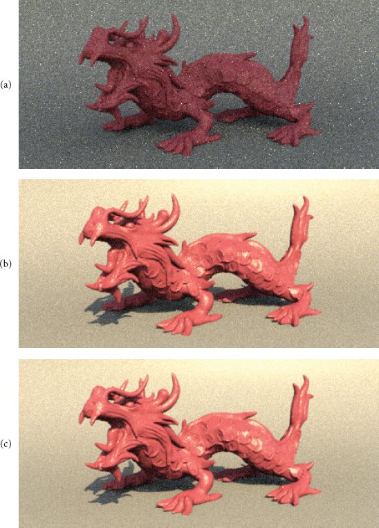
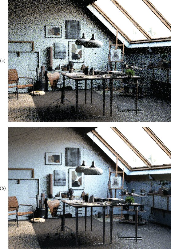
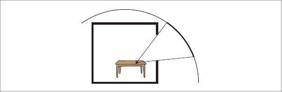
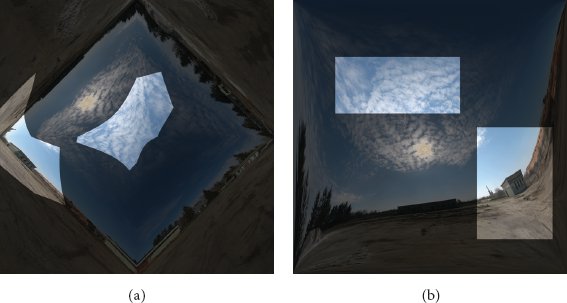

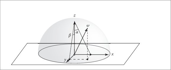
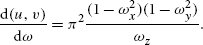
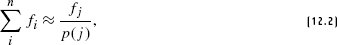
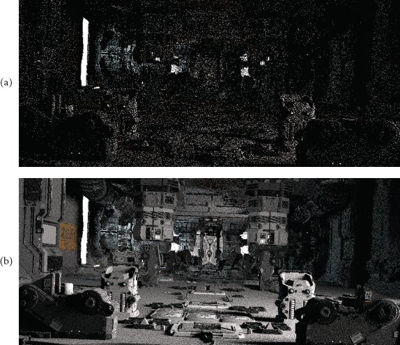

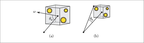
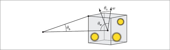
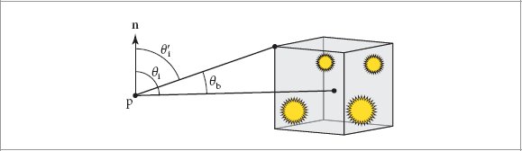
 that gives a lower bound on the angle between the incident lighting direction and the surface normal can be found by subtracting θb, the angle that the bounding box subtends with respect to the reference point p, from θi, the angle between the surface normal and the vector to the center of the box.
 directly using the sines and cosines of the two contributing angles.
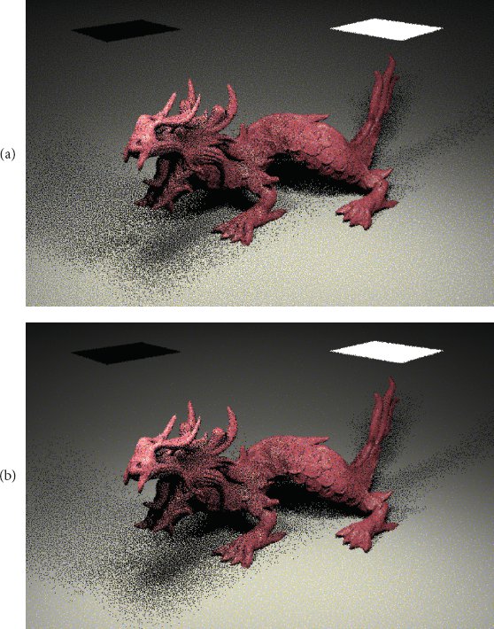
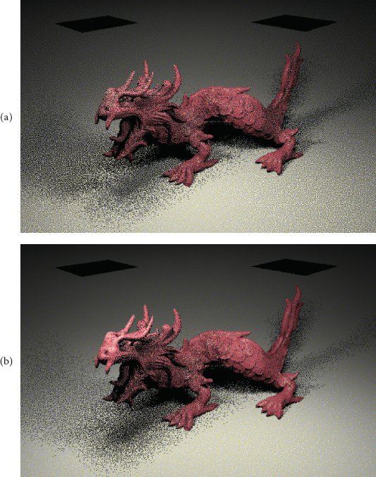
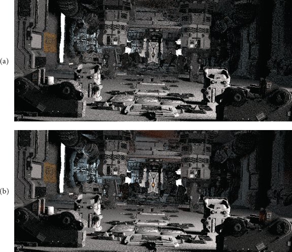
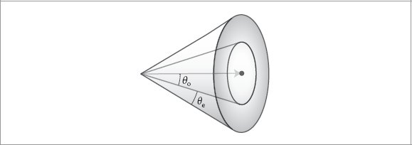
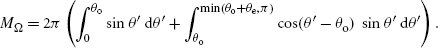
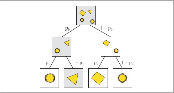
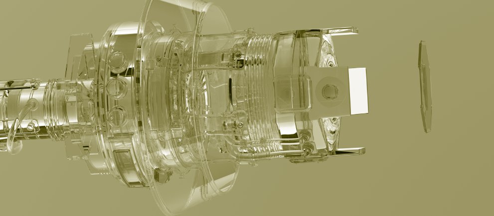

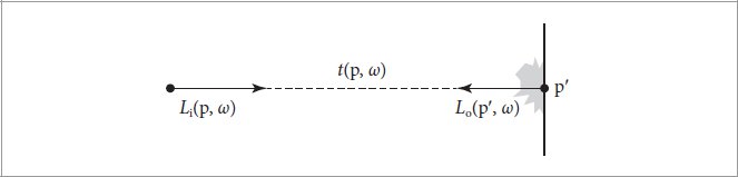

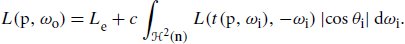
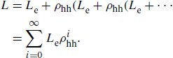

 . We can also write the BSDF at p′ as
 and
and  (
(
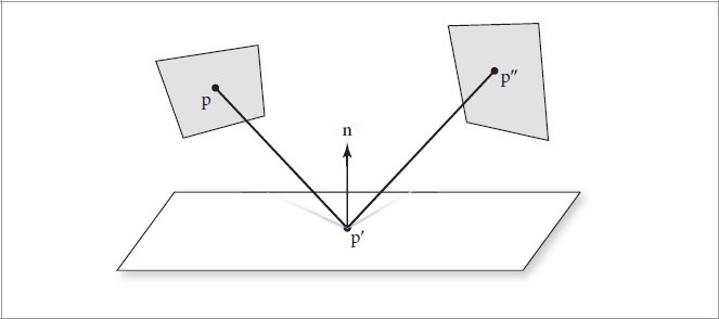
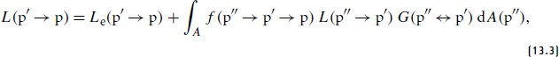
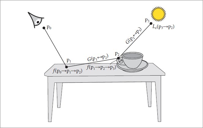
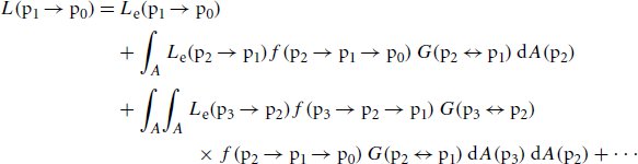
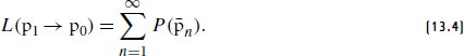
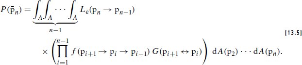
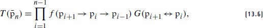
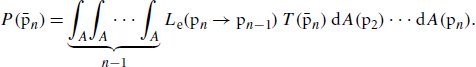
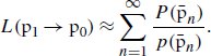
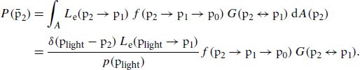
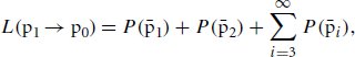
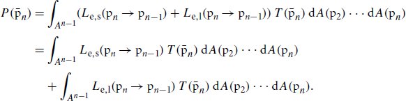
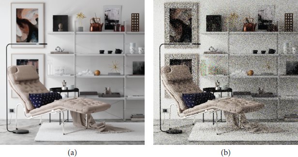
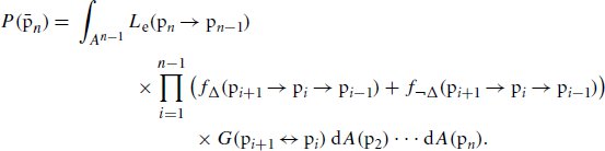
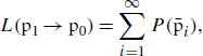
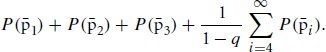
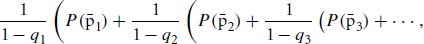
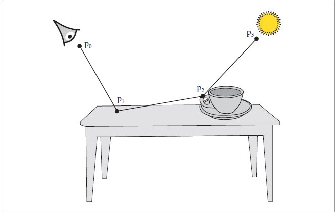

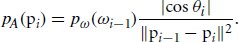
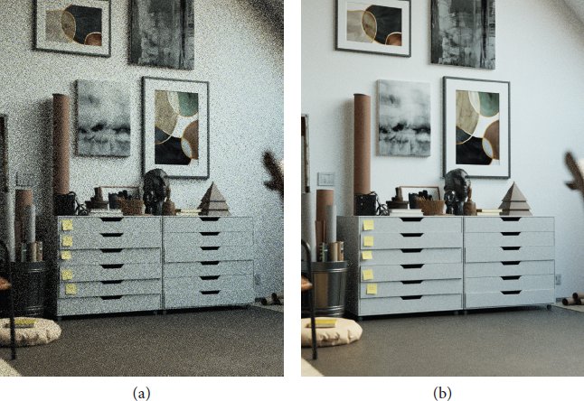
 and
and 

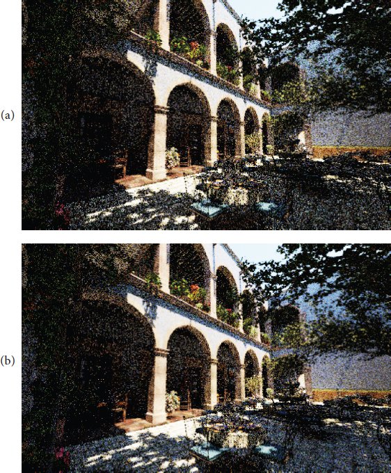

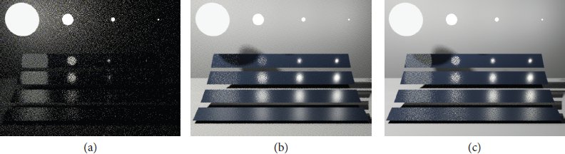
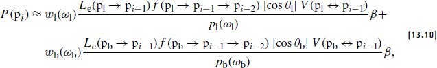

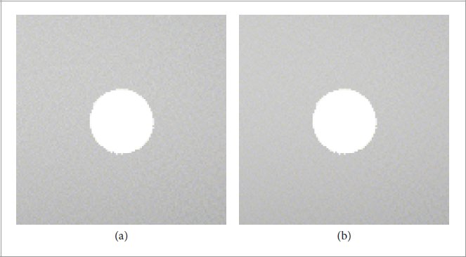
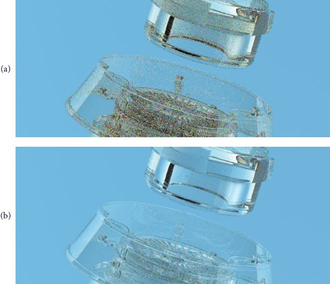
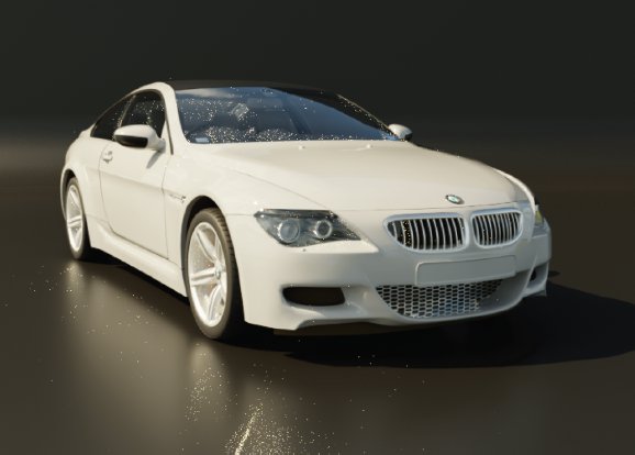
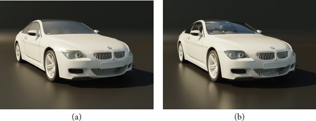


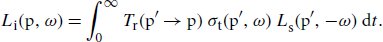
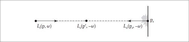

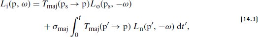

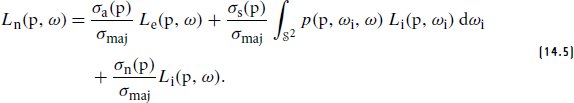
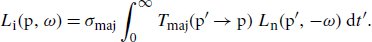
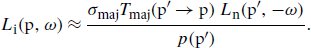
 is
is 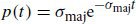 , and so the estimator simplifies to
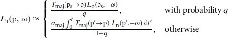

 and its endpoint as pi, the transmittance can be written as
 is the transmittance function for the ith segment and the point p′ is the endpoint of the nth segment. (This relationship uses the multiplicative property of transmittance from
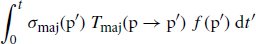
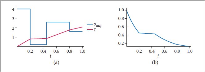
 , it is useful to rewrite the integral to be over the individual majorant segments, which gives
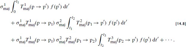
 from
from  distribution p1; if
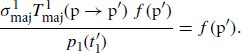
 from
from  distribution, starting at t1. If the sampled point is before the segment’s endpoint,
  , then we have the estimator
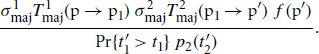
 is equal to
  , the estimator for the second term again simplifies to f (p′). Otherwise, following this sampling strategy for subsequent segments similarly leads to the same simplified estimator in the end. It can furthermore be shown that the probability that no sample is generated in any of the segments is equal to the full majorant transmittance from 0 to t, which is exactly the probability required for the surface/volume estimator of
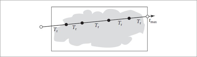
 . Separate cases handle a sample that is within the current majorant segment and one that is past it.
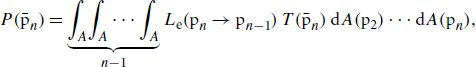
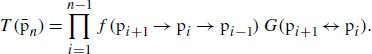
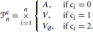
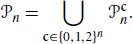
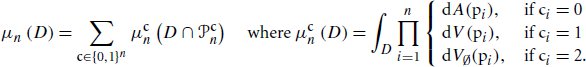
 can now be written as

 can then be defined as:
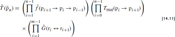
 and generalized geometric term Ĝ. The former simply falls back to the BSDF, phase function (multiplied by σs), or a factor that enforces the ordering of null-scattering vertices, depending on the type of the vertex pi. Note that the first two products in
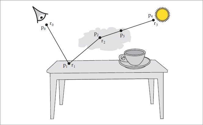
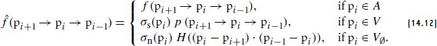
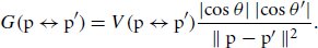

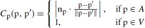
 can be defined for a path
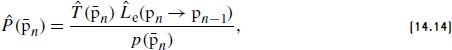
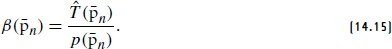
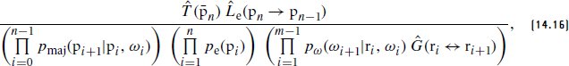
 , and the exponential factors cancel out the Tmaj factors in
  , each one leaving behind a 1/σmaj factor. Expanding out
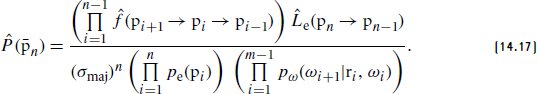
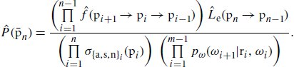
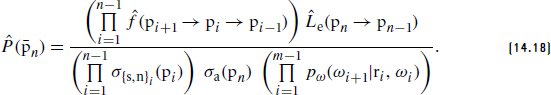
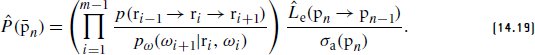
 or the path throughput weight β(
 from a wavelength-dependent PDF based on the first wavelength and then evaluate f at all the wavelengths, we have the estimators
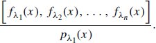
 that was used for sampling matches
  well, it may be a poor match for f at the other wavelengths. It may not even be a valid PDF for them, if it is zero-valued where the function is nonzero. However, falling back to integrating a single wavelength at a time would be unfortunately inefficient, as shown in
  , then the final estimator for λ′ will include a factor of
  that can be arbitrarily large.
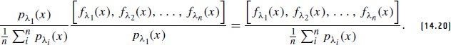
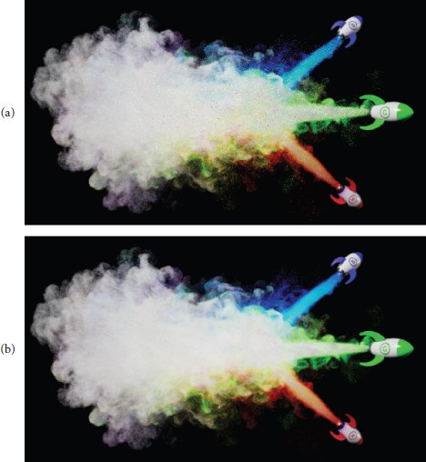
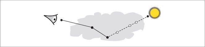
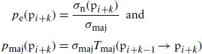
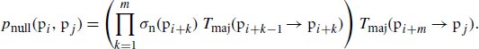


 sampled using light path sampling, the two-sample MIS estimator is
 and
and  do as well, following
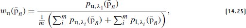
 function in the numerator replaced with
  .
.
 in the denominator of the first term of the two-sample MIS estimator,
  factor in the second term of the estimator and in the wl weight. It is tempting to cancel these out; in that case, the path state to be tracked by the integrator would consist of
  and the wavelength-dependent probabilities pu(
 maintained independently, a series of specular bounces could lead to overflow. (Many null-scattering events along a path can cause similar problems.)
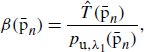

 for paths that end with a shadow ray from light path sampling and the unidirectional path probability otherwise. (Later in the implementation, we will take advantage of the fact that these two probabilities are the same until the last scattering vertex, which in turn implies that whichever of them is chosen for ppath does not affect the values of
  and
and  .)
.) , then MIS weights like those in
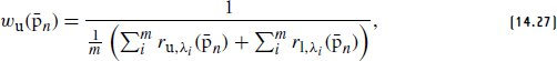
 .
.
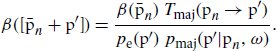
 . Because we are always sampling absorption (at least as far as including emission goes), pe is 1 here.
 , and the probability for sampling real scattering, σs(p′)/σmaj. The σmaj values cancel.
 for this vertex here. The associated directional PDF for light sampling at this vertex will be incorporated into
  factor included. The other factors in
  for the path up to the scattering vertex. Thus,
  . This allows multiplying
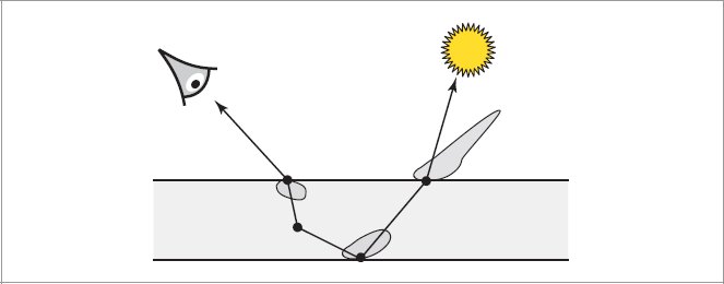
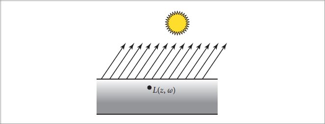


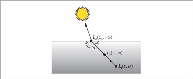


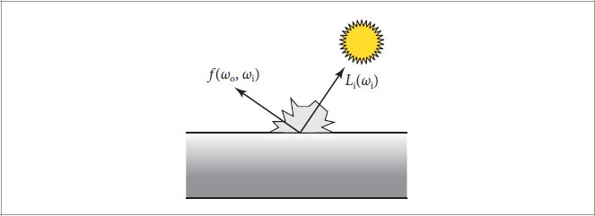
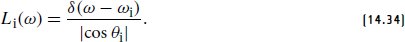

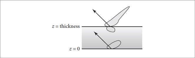
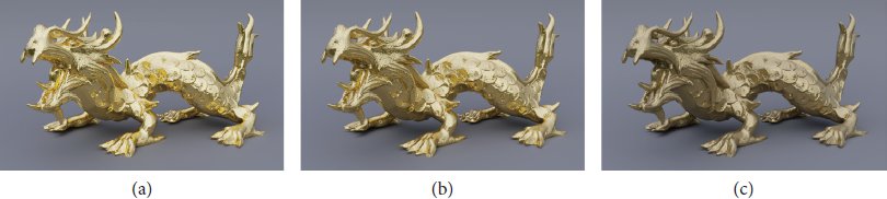
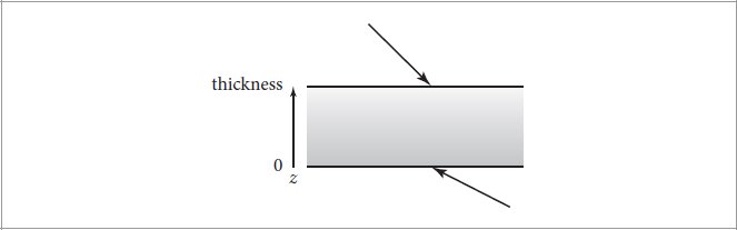
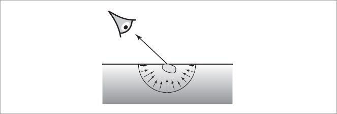

 is the hemisphere inside the medium (see
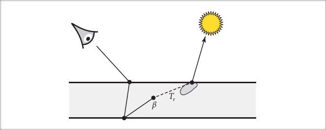
 and a top layer that both reflects light with BRDF
  and transmits it with BTDF
  , with an overall BSDF
  . If those BSDFs have associated PDFs p and if scattering in the medium is neglected, then the overall PDF is
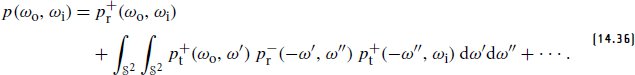
 , and so forth (see
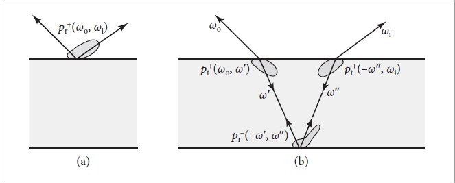
 and its negation gives one of the two directions for
  . A second direction ω″ is used for
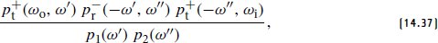
 will always be zero unless ω″ was sampled according to its PDF.
 ’s sampling method, conditioned on ωo, and if ω″ is sampled using
  as the estimate; the effect of
  .
.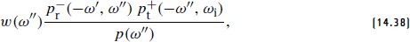
 .
. factor cancels out as well and the estimator is
  times the MIS weight.
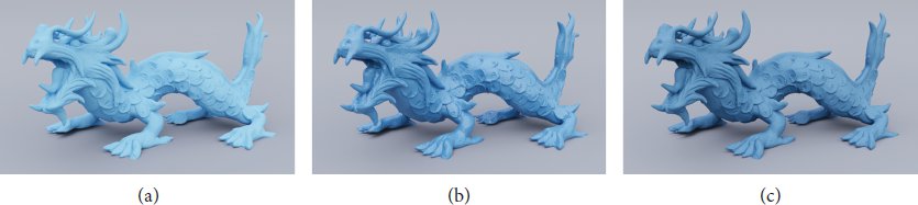
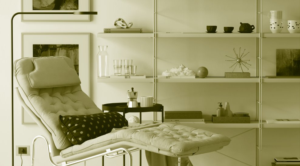
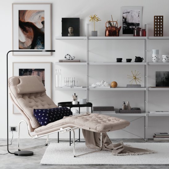
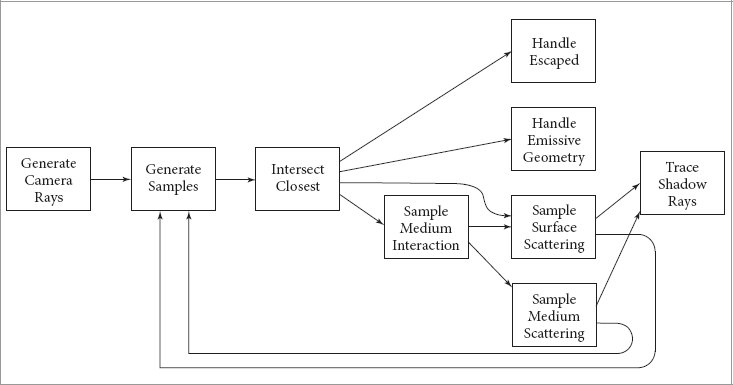
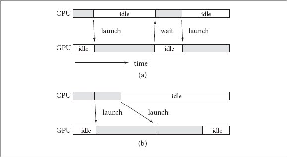
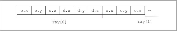
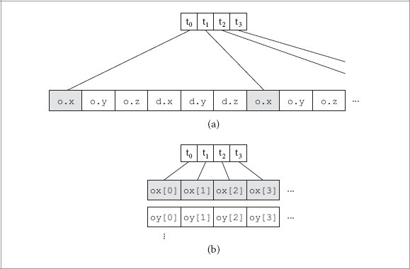
 and path sampling PDFs are updated along the way. In the end, if the ray is neither scattered nor absorbed, then work is added to queues in the same manner as for rays that are not passing through media in the closest hit shader.
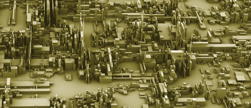
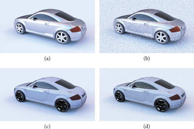


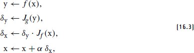

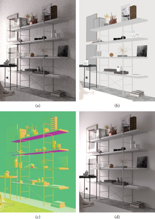

 . Thus, the average
  value is 1, which will be convenient in the following.
 worth of probability mass. With one less bin to initialize and that much less probability to distribute, we have the same average probability over the remaining bins. That brings us to the same setting as the starting condition: some of the remaining items in the list must be above the average and some must be below, unless they are all equal to it.
 of
of  , it certainly has enough probability to fill the remainder of the bin—we just need
  of it.
 worth of the scaled probability mass. The remainder,
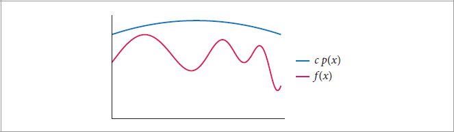

 . If the method is applied to generate samples in hyperspheres in the general n-dimensional case, however, the volume of an ndimensional hypersphere goes to 0 as n increases, and this approach becomes increasingly inefficient.


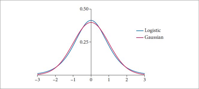
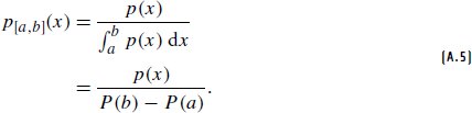

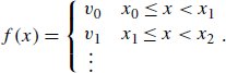
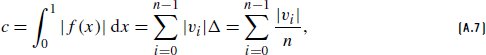
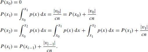
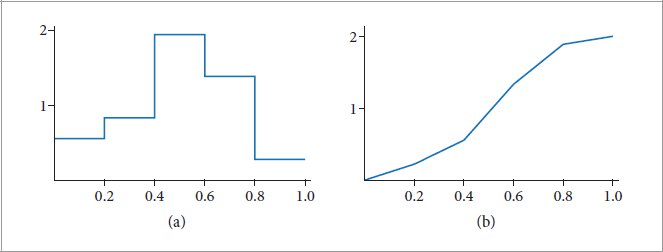
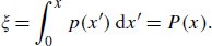
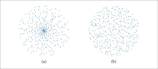
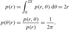


 of the unit square of uniform random samples in each direction. In general, we would prefer a mapping that did a better job at mapping nearby (ξ1, ξ2) values to nearby points on the disk.


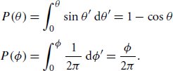
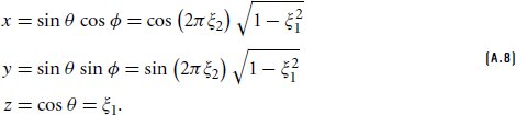
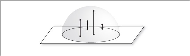
 method.
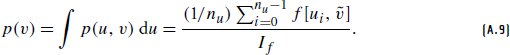

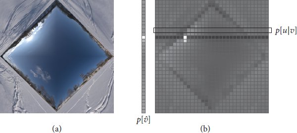
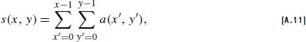
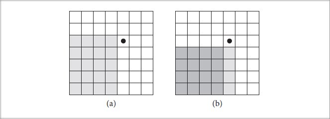
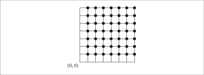
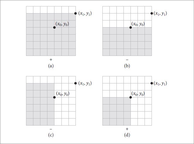
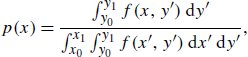
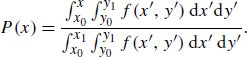
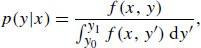
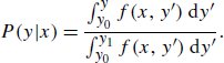

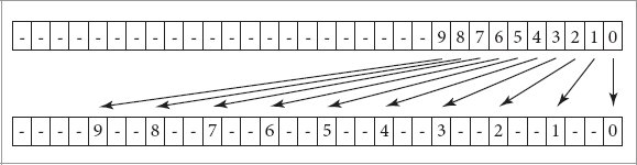
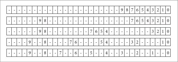
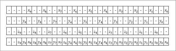
 due to cancellation error. It can be rewritten algebraically into a more stable form:
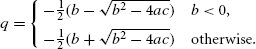
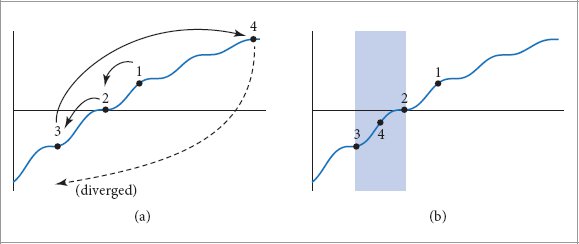
 , then the sample variance could be estimated as
 . In turn, S/(n − 1) gives the sample variance.

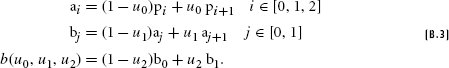
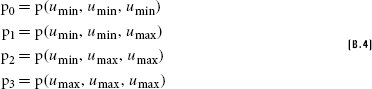


 .exr is a feature worth devoting attention to.)
 is U+5149.
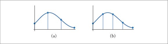

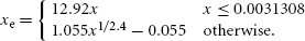
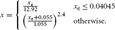

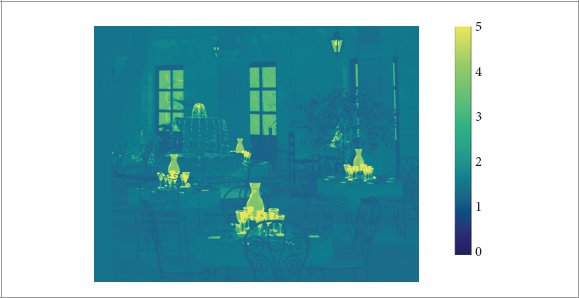
 〉,
〉,  〉,
〉,